This study evaluates the performance of various meta-analytic methods for binary outcomes, with the OR serving as the effect measure [20]. The models compared include four binomial-normal GLMMs (two for frequentist analysis, two for Bayesian analysis) [11, 17], two beta-binomial models (one for frequentist analysis, the other for Bayesian analysis) [3, 12], the generalized estimating equations (GEE) with three different working correlation matrices [16, 21, 22], and the hypergeometric-normal GLMM [13]. Table 1 summarizes all the models considered.
This section describes the details of the statistical methods that were compared. Indexes i = 1, 2, … k to denote the studies, and j = 0, 1 denote the treatment status (where j = 0 and j = 1 indicate the control and the treatment arms, respectively). \(\:{\pi\:}_{ij}\) and \(\:{r}_{ij}\) denote the true event risk and the event counts in the ith study and the jth treatment arm, respectively.
Binomial-normal GLMM (GLMM-A, GLMM-B)
There are various parameterisation methods for GLMMs, which can be estimated using either a frequentist or a Bayesian approach. Turner et al. [23] explored the potential of GLMMs for meta-analysis of RCTs with binary outcomes, using both summary (e.g. log-OR) and individual data. Simmonds and Higgins [24] have documented the general GLMM framework for different types of meta-analysis. Standard GLMMs used in meta-analyses include the random-slope GLMMs and the random intercept and slope GLMMs [11]. For the random-slope GLMMs, the true underlying treatment effect is assumed to differ for each trial, but the baseline risk of the event in each study is fixed. Assuming that \( \:r_{{ij}} |\pi \:_{{ij}} (n_{{ij}} ,\pi \:_{{ij}} ) \), the meta-analytic model can be written as: [25]
$$\log it\left( {{\pi _{ij}}} \right)={\gamma _i}+{\theta _i}~I\left( {j=1} \right)$$
(1)
Where the \(\:{\gamma\:}_{i}\:\)denotes the log odds in the control group of study i, and I (Ÿ) is the indicator function. \( \:\theta \:_{i} \left( {\theta \:,\tau \:^{2} } \right) \), where \( \:\theta \:_{i} \) is the true underlying log OR for the ith study, θ is the true mean log-OR, and \(\:{\tau\:}^{2}\) is the between-study treatment effect variance. The random-intercept and slope GLMM employ both a random study effect \( \:\gamma \:_{i} \left( {\gamma \:,\:\sigma \:^{2} } \right) \) and a random treatment effect\( \:\:\theta \:_{i} \left( {\theta \:,\tau \:^{2} } \right).\: \)An equivalent way of expressing this model is \(\:logit\left({\pi\:}_{ij}\right)={\gamma\:}_{i}+\theta\:\:I\left(j=1\right)+{ϵ}_{i}\:I\left(j=1\right)\), where \( \in _{i} \sim \left( {0,\tau \:^{2} } \right) \).
Jackson et al. [11] and Bakbergenuly and Kulinskaya [26] investigated the performance of an alternative parameterization of this model, where Eq. (1) is replaced by:
$$\log it\left( {{\pi _{ij}}} \right)={\gamma _i}+\theta I\left( {j=1} \right)+\left[ {I\left( {j=1} \right) – \frac{1}{2}} \right]{ \in _i}$$
(2)
These parameterizations for Eqs. (1) and (2) assume different bivariate covariance structures in terms of the joint distribution of \(\:logit\left({\pi\:}_{i0}\right)\) and \(\:logit\left({\pi\:}_{i1}\right)\)[26]. Equation (2) also can model the intercepts \(\:{\gamma\:}_{i}\) as fixed or random.
This has been criticized regardless of whether the intercepts \(\:{\gamma\:}_{i}\:\)are modelled as fixed or random in the two parameterizations. Modelling a fixed study-specific intercept can lead to a Neyman–Scott problem [27], while modelling a random intercept may result in bias from the recovery of intertrial information [28]. Jackson et al. [11] conducted extensive simulations and found that the bias from the recovery of intertrial information is very small when the intercepts \(\:{\gamma\:}_{i}\) are modelled as random. Thus, this bias is not a serious concern. Ju et al. [29] found that modelling the intercepts \(\:{\gamma\:}_{i}\) as random had some advantages in dealing with heterogeneous studies, such as better coverage and less susceptibility to bias of treatment effect variance between studies. Jansen et al. [30] suggested that the GLMMs with fixed intercepts should be used cautiously in rare events meta-analyses. Therefore, the random-intercept and slope GLMM is used in this study. The random intercept and slope GLMMs using the parameterisations of Eqs. (1) and (2) are denoted GLMM-A and GLMM-B, respectively.
Binomial-normal hierarchical model (BNHM-1, BNHM-2)
GLMM-A and GLMM-B can also be fit within a Bayesian framework, and the two models have similar statistical performance under Bayesian estimation [31]. In this study, we opted to estimate GLMM-A using a Bayesian framework where we modelled the intercept \(\:{\gamma\:}_{i}\) as fixed effect. Under a Bayesian framework, the GLMM-A also called the BNHMs [15], we denoted it as BNHM-1. The BNHM-1 was first discussed by Bhaumik et al. [10] In a fully Bayesian analysis, prior distributions must be specified for the unknown parameters that include the \(\:{\gamma\:}_{i}\), \(\:\theta\:\), and \(\:{\tau\:}^{2}\).
The likelihood function for the second Bayesian model (BNHM-2) is also based on the GLMMs and was introduced by Smith et al. [15] Assuming that \( \:r_{{ij}} |\pi \:_{{ij}} (n_{{ij}} ,\pi \:_{{ij}} ) )\), the unknown parameter \(\:{\pi\:}_{ij}\) is modeled as:
$$\log it\left( {{\pi _{ij}}} \right)={\gamma _i}+{\theta _i}{z_{ij}}$$
(3)
where, \(\:{z}_{ij}=0.5\:\)(j = 1) or \(\:{z}_{ij}=-0.5\) (j = 0), and \( \:\theta \:_{i} \left( {\theta \:,\tau \:^{2} } \right) \). Prior distributions must also be specified for the unknown parameters \(\:{\gamma\:}_{i}\), \(\:\theta\:\) and \(\:{\tau\:}^{2}.\).
The difference between Eqs. (1), (2), and (3) is that we assume different bivariate structures in the control and treatment groups for each study. From Eq. (3), we have
$$\left( {\begin{array}{*{20}{c}} {\log it\left( {{\pi _{i0}}} \right)} \\ {~\log it\left( {{\pi _{i1}}} \right)} \end{array}} \right)\sim N\left( {\left( {\begin{array}{*{20}{c}} {{\gamma _i} – 0.5\theta } \\ {~{\gamma _i}+0.5\theta } \end{array}} \right),~\left( {\begin{array}{*{20}{c}} {{\tau ^2}/4}&{ – {\tau ^2}/4} \\ { – {\tau ^2}/4}&{{\tau ^2}/4} \end{array}} \right)} \right)$$
(4)
From Eq. (2), we have
$$\left( {\begin{array}{*{20}{c}} {\log it\left( {{\pi _{i0}}} \right)} \\ {~\log it\left( {{\pi _{i1}}} \right)} \end{array}} \right)\sim N\left( {\left( {\begin{array}{*{20}{c}} {{\gamma _i}} \\ {~{\gamma _i}+\theta } \end{array}} \right),~\left( {\begin{array}{*{20}{c}} {{\tau ^2}/4}&{ – {\tau ^2}/4} \\ { – {\tau ^2}/4}&{{\tau ^2}/4} \end{array}} \right)} \right)$$
(5)
From Eq. (1), we have
$$\left( {\begin{array}{*{20}{c}} {\log it\left( {{\pi _{i0}}} \right)} \\ {~\log it\left( {{\pi _{i1}}} \right)} \end{array}} \right)\sim N\left( {\left( {\begin{array}{*{20}{c}} {{\gamma _i}} \\ {~{\gamma _i}+\theta } \end{array}} \right),~\left( {\begin{array}{*{20}{c}} 0&0 \\ 0&{{\tau ^2}} \end{array}} \right)} \right)$$
(6)
Here, the two BNHMs modelled the intercepts \(\:{\gamma\:}_{i}\) as fixed effect, we assume a diffuse normal prior on \( \:\gamma \:_{i} \left( {\gamma \:_{0} ,10^{2} } \right) \) centered around \(\:{\gamma\:}_{0}=\sum\:_{i=1}^{k}{\gamma\:}_{ie}/k\), where \(\:{\gamma\:}_{ie}\) denotes the empirical log-odds for the control group in study i [32, 33]. Continuity corrections (adding 1/2) would be utilized to calculate the estimates of \(\:{\gamma\:}_{ie}\) for studies with zero-events.
Günhan et al. [17] suggested that the use of a weakly informative prior (WIP) for the treatment parameter \(\:\theta\:\) displays good statistical properties compared to a non-informative prior (NIP). Following their suggestions, a normal prior with a mean of 0 and standard deviation of 2.82 is assigned to the treatment parameter \(\:\theta\:\), which is consistent with empirically observed effect estimates that were derived from a set of 37,773 meta-analysis datasets from the Cochrane Database of Systematic Reviews (CDSR). [17]
A WIP is also assigned for the heterogeneity parameter , that is, a half-normal prior with scale of 0.5 [\( \:\tau \:\left( {0.5} \right) \)] [19, 34]. The heterogeneity parameter prior has a median of 0.34, with an upper 95% quantile of 0.98. Values for of 0.30, 0.75 and 1 represent reasonable, fairly high, and fairly extreme heterogeneities, respectively [35]. Thus, \( \:\tau \:\left( {0.5} \right) \) captures heterogeneity values typically seen in meta-analyses of heterogeneous studies.
Hypergeometric-normal model (Nchg)
This model was first proposed by Van Houwelingen et al. [13], Stijnen et al. [24] discussed its potential advantages in the context of rare events meta-analyses. The Nchg assumes that \( \:r_{{ij}} |\pi \:_{{ij}} (n_{{ij}} ,\pi \:_{{ij}} ) \). Upon the condition that the total number of events in the study, all marginal totals of the 2-by-2 tables \(\:{r}_{i}=\:{r}_{i0}+{r}_{i1}\) are fixed, then \(\:{r}_{i1}|{r}_{i}\) follows a noncentral hypergeometric distribution, and we have:
$$f\left( {{r_{i1}}~|{r_i},{n_{ij}},{\theta _i}~} \right)=\frac{{\left( {\begin{array}{*{20}{c}} {{n_{i1}}} \\ {{r_{i1}}~} \end{array}} \right)\left( {\begin{array}{*{20}{c}} {{n_{i0}}} \\ {{r_{i0}}~} \end{array}} \right)\exp \left( {{\theta _i}{r_{i1}}} \right)}}{{\mathop \sum \nolimits_{{m \in M}} \left( {\begin{array}{*{20}{c}} {{n_{i1}}} \\ {m~} \end{array}} \right)\left( {\begin{array}{*{20}{c}} {{n_{i0}}} \\ {{r_i} – m~} \end{array}} \right)\exp \left( {{\theta _i}m} \right)}}$$
(7)
Where \(\:{\theta\:}_{i}\) is the true underlying log OR for the ith study, the summation m is over the \(\:{r}_{i1}\) values that are permissible under the table marginal totals. Assuming that \( \:\theta \:_{i} \left( {\theta \:,\tau \:^{2} } \right) \), \(\:{\tau\:}^{2}\) is the between-study treatment effect variance, this is made a random-effects model. One favourable property of this model is that there is no need to specify how additional nuisance parameters (such as the intercepts in GLMM-A and GLMM-B) are modelled, which ensures consistency of the maximum likelihood estimators of \(\:\theta\:\) and \(\:{\tau\:}^{2}\), where \(\:\theta\:\:\)denote the pooled log-OR and \(\:{\tau\:}^{2}\) is the between-study treatment effect variance [30].
Beta-binomial model by Kuss (Betabin)
The first model, proposed by Kuss (Betabin) [3], is fitted within a frequentist framework. Assuming that \( \:r_{{ij}} |\pi \:_{{ij}} (n_{{ij}} ,\pi \:_{{ij}} ) \), that the \( \:\pi \:_{{ij}} (a_{j} ,b_{j} ) \), with \(\:{a}_{j}>0\) and \(\:{b}_{j}>0\). As a consequence, \(\:E\left({\pi\:}_{ij}\right)={\mu\:}_{j}={a}_{j}/({a}_{j}+{b}_{j})\). Then, the number of events in the control and treatment group follows a beta-binomial distribution. The Betabin by Kuss is applied in conjunction with a logit link function, the \(\:{logit(\mu\:}_{j})\) is predicted through an intercept and an indicator of the experimental group membership\(\:\:I\left(j=1\right)\), yielding [3]:
$$\log it({\mu _j})=\gamma +\theta I\left( {j=1} \right)$$
(8)
Where θ denotes the pooled log-OR, \(\:\gamma\:\) represents the average log odds of the control group.
Beta hyperprior model (Beta-hyperprior)
The second model, proposed by Hong et al. (Beta-hyperprior) [12], is estimated within a Bayesian framework. Using the likelihood \( \:r_{{ij}} |\pi \:_{{ij}} (n_{{ij}} ,\pi \:_{{ij}} ) \), the Beta-hyperprior model considers trials’ treatment-specific risks as follows [12]:
$${\pi _{ij}}\sim Beta\left( {{U_j}{V_j},~\left( {1 – {U_j}} \right){V_j}} \right)$$
(9)
where \(\:E\left({\pi\:}_{ij}|{U}_{j},{V}_{j}\right)={U}_{j}\) and \(\:Var\left({\pi\:}_{ij}|{U}_{j},{V}_{j}\right)=\frac{{U}_{j}\left(1-{U}_{j}\right)}{{V}_{j}+1}\). Comparing Eq. (9) with Eq. (8), it is found that the two models are the same, just parametrized differently. In the case of the common Beta (\(\:{\alpha\:}_{j},\:{\beta\:}_{j}\)) parameterization, \(\:{U}_{j}=\frac{{\alpha\:}_{j}}{{\alpha\:}_{j}+\:{\beta\:}_{j}}\) and \(\:{V}_{j}=\:{\alpha\:}_{j}+\:{\beta\:}_{j}\). Thus, \(\:{U}_{j}\) denotes the true mean probability of having an event with treatment j. Heterogeneity in the trials’ treatment-specific risk is measured by \(\:\frac{{U}_{j}\left(1-{U}_{j}\right)}{{V}_{j}+1}\). Similar to Hong et al. [12] a vague Beta (1, 1) and inverse-Gamma (10, 0.01) is assigned prior to \(\:{U}_{j}\) and \(\:{V}_{j}\), respectively. OR can be obtained by \(\:{[U}_{1}/(1-{U}_{1}))/{(U}_{0}/(1-{U}_{0}\left)\right]\).
Generalized estimating equations (GEE-UN, GEE-IN, GEE-EX)
The model GEE, proposed by Liang and Zeger et al. [21, 22], allows longitudinal analysis according to the marginal model [22, 36]. A working correlation matrix is used to define the GEE and obtain an efficient variance estimate [21]. Curtin [37, 38] presented a meta-analysis method based on GEE regression to combine aggregated results of crossover and parallel trials. For meta-analyses, each study is a cluster, and the working correlation matrix indicates the probability correlation of an event in the treatment and control groups within a study. The GEE in a meta-analysis is [16]:
$$\log it\left( {E\left[ {{y_{ij}}} \right]={\pi _{ij}}} \right)=j\theta $$
(10)
Where θ is the true mean log-OR. The logit () function links the treatment variable j to the marginal expectation of the outcome \(\:{y}_{ij}\), and \(\:{y}_{ij}\) is the observed event risk in the ith study and the jth treatment group. A function g relates the expectation of the outcome \(\:{y}_{ij}\:\)to its variance \(\:{\nu\:}_{s}\) by \(\:{\nu\:}_{s}=v\left({y}_{ij}\right)\varphi\:=g\left({\pi\:}_{ij}\right)\varphi\:\), where \(\:v\left({y}_{ij}\right)\) is the variance function, and \(\:\varphi\:\) is a scale parameter. The variance-covariance matrix within studies for \(\:{y}_{i}=\left({y}_{i0},{y}_{i1}\right)\) can be written \(\:{\varvec{V}}_{i}=\) \(\:\varphi\:{A}_{i}^{1/2}R\left(a\right){A}_{i}^{1/2}\), where \(\:R\left(a\right)\) denotes the working correlation matrix, and \(\:{A}_{i}\) is the usual estimate of the variance based on the information matrix [39]. There are seven different working correlation matrix types [21], three of which are suitable for meta-analysis [16], including the independent structure, exchangeable correlation, and unstructured correlation, denoted by GEE-IN, GEE-EX, and GEE-UN, respectively.
SimulationSimulation setup
A number of scenarios are evaluated by varying the control event rate \(\:{p}_{c}\), the value of the treatment effect log OR, the number of studies k, the between-study deviation . More specifically, these values were varied as follows:
The control event rate: To reflect the rare events cases, the control event rate\(\:\:{p}_{c}\) is taken as 0.01 or 0.05.This definition of rare events was also used by Jackson et al. [11], Xu et al. [16], and Jansen et al. [30]
The treatment effect log OR: This value varied as \(\:\theta\:\in\:\left\{-0.93,\:-0.34,\:0,\:0.46,\:1.05\right\}\), which represents ORs of 0.39 (\(\:\theta\:=-0.93\)), 0.71 (\(\:\theta\:=-0.34\)), 1 (\(\:\theta\:=0\)), 1.58 (\(\:\theta\:=0.46\)), and 2.86 (\(\:\theta\:=1.05\)). These values were inspired by a reanalysis of Cochrane reviews conducted by Beisemann et al. [40] In their reanalysis, they obtained a mean log-RR of 0.06 with a standard deviation of 0.6 across Cochrane reviews. We assumed that a reanalysis of the log-OR would yield similar numbers, as the log-RR and log-OR are very similar for rare events. The log-OR values, specifically − 0.93, -0.34, 0, 0.46, and 1.05, roughly correspond to this empirical distribution’s 5%, 25%, 50%, 75%, and 95% quantiles.
Number of studies per meta-analysis: The number of simulated studies for each meta-analysis is taken as 5, 10, and 30. Jansen et al. [30] used these values, which roughly mirror the 75%, 90%, and 99% quantiles of the empirical distribution of the number of studies reported in the review by Davey et al. [41]
Number of patients in the control group of a single study: Following Xu et al. [16] the sample sizes in the control arm (\(\:{n}_{c})\:\)are simulated from a log-normal distribution with mean 3.3537 and standard deviation 0.9992.
Number of patients in the treatment group of a single study: the sample size in the treatment group (\(\:{n}_{t})\) is derived from the equation: \(\:{n}_{t}\)=\(\:{n}_{c}\)× R, the empirical ratio (R) is a uniform distribution: \(\:R\:\sim\:uniform(0.84,\:2.04)\) [16].
Degree of heterogeneity: Four different settings [0.05 (small), 0.30 (reasonable), 0.75 (fairly high), and 1 (fairly extreme)] are used to generate small to fairly extreme between-study heterogeneity [42].
Simulation scenarios
Combining the four design factors (event probability in the control group \(\:{p}_{c}\), size of treatment effect log OR, number of studies per meta-analysis k, between-study deviation ) results in a total of 120 simulation scenarios. Table 2 presents the simulation settings. For each fixed scenario, we first simulated 10,000 meta-analyses. Then, the meta-analyses with a zero total event count in a single arm or in both arms were excluded, because the GLMM-A, GLMM-B, Betabin, GEE-UN, GEE-IN, and GEE-EX cannot pool the results when the total event count is zero in a single or in both arms [16, 29, 30]. The proportion of simulated datasets that were dropped from the simulation can be found in the Supporting Information (Figures S1–S2). The proportion of excluded datasets ranged from 0 to 25%. The proportion was higher, ranging from 3 to 25%, when both the number of studies and the control event rate were small (\(\:{p}_{c}=0.01\) and k = 5). For the other simulated settings, the proportion was low, with most of the settings less than 5%. The Supporting Materials also shows the average percentage of single- and double-zero events datasets (Figures S3-S4), and the percentage of simulated datasets with a total of at least 10 events in one or both arms (Figures S5-S6).
Data generation
We used the “pRandom” to generate grouped data for the current simulations [43]. Set the values for (log- OR), (between-study heterogeneity), k (number of studies), and \(\:{p}_{c}\) (event rate in the control group). For i = 1, 2, … k:
(i)
Generate the control group sample size: \(\:{n}_{i0}\:\sim\:LN(3.3537,\:0.9992)\).
(ii)
Generate the sample size ratio: \(\:R\:\sim\:uniform(0.84,\:2.04)\)
(iii)
Compute the treatment group sample size: \(\:{n}_{i1}={n}_{i0}\times\:R\).
(iv)
Compute the average treatment group logits\(\:\:{p}_{t}\): \(\:{p}_{t}={p}_{c}\text{exp}\left(\theta\:\right)/\{1-{p}_{c}+{p}_{c}\text{exp}\left(\theta\:\right)\}\).
(v)
Compute the \(\:logit\left({p}_{t}\right)\) and \(\:logit\left({p}_{c}\right)\), where\(\:\:logit\left(x\right)=\text{l}\text{o}\text{g}\left\{\frac{x}{1-x}\right)\}\).
(vi)
Generate study-specific control and treatment logits: \( \:logit(p_{{ij}} )\left\{ {{\text{logit}}\left( {p_{j} } \right),\:\tau \:/\sqrt 2 } \right\} \).
(vii)
Compute the study-specific control and treatment event rate: \(\:{p}_{ij}=\text{e}\text{x}\text{p}\text{i}\text{t}\left\{{logit(p}_{ij}\right)\}\).
(viii)
Generate the study events: \( r_{{ij}} \sim Binomial\left( {n_{{ij}} ,p_{{ij}} } \right) \).
Model fit
The simulations were performed using R (version 4.1.2, R Foundation for Statistical Computing, Vienna, Austria). The glmer() function of the lme4 package (version 1.1–27.1) was used to fit GLMM-A and GLMM-B [30, 44]. GEE-UN was estimated using the gee package (version 4.13-25). GEE-IN and GEE-EX were estimated using the geepack package (version 1.3.9). Nchg was estimated using the metafor package (version 3.0–2). For Betabin, the code provided by Beisemann et al. [40] was used, replacing the log-link with a logit-link to obtain estimates of the log-OR instead of the log-RR. This code uses the dbbinom() function from the extraDistr package (version 1.9.1) to model the beta-binomial likelihood, and then uses optim() function to maximize the likelihood.
All Bayesian methods (BNHM-1, BNHM-2, and Beta-hyperprior) were computed using Hamiltonian Monte Carlo algorithms, as implemented in the RStan package (version 2.21.2). Four chains were fitted for each model, and each was run for 5,000 iterations, of which the first half was removed as burn-in, and the remaining ones were thinned by 1. Convergence was deemed to have occurred when \(\:\widehat{R}\) (potential scale reduction factor) was no greater than 1.1 for all parameters [45].
Evaluating simulation performance
The model performance was evaluated by assessing on the OR scale:
(i)
Median percentage bias [PB, defined as \(\:median\left(\frac{\:\widehat{\varvec{\theta\:}}-\theta\:}{\theta\:}\right)\times\:100\text{\%}\)],
(ii)
Median width of 95% confidence or credible interval (95% CI or CrI, defined as \(\:median({\widehat{\varvec{\theta\:}}}_{upper}-{\widehat{\varvec{\theta\:}}}_{lower}\)),
(iii)
Root-mean-square-error (RMSE, defined as\(\:\:\sqrt{\frac{{\sum\:}_{i}^{{n}_{est}}{|{\widehat{\theta\:}}_{i}-\theta\:|}^{2}}{{n}_{est}}}\) ).
(iv)
Empirical coverage (defined as\(\:\:\frac{{{\sum\:}_{i}^{n}I(\widehat{\theta\:}}_{i})}{n}\times\:100\text{\%}\) ).
Where \(\:\widehat{\varvec{\theta\:}}=\)\(\left({\widehat{\theta\:}}_{1},{\widehat{\theta\:}}_{2},\dots\:,{\widehat{\theta\:}}_{n}\right)\), \(\:{\widehat{\varvec{\theta\:}}}_{lower}=\)\(({\widehat{\theta\:}}_{1,lower},{\widehat{\theta\:}}_{2,lower},\dots\:,{\widehat{\theta\:}}_{n,lower})\), and \(\:{\widehat{\varvec{\theta\:}}}_{upper}=\)\(\left({\widehat{\theta\:}}_{1,upper},{\widehat{\theta\:}}_{2,upper},\dots\:,{\widehat{\theta\:}}_{n,upper}\right).\) \(\:{\widehat{\theta\:}}_{i}\), \(\:\theta\:\), and \(\:{I(\widehat{\theta\:}}_{i})\) denote the estimated treatment effect for the ith simulated dataset, the true treatment effect, and the indicator function (equal to 1 when the true treatment effect was covered by the boundaries, and 0 when not covered by the boundaries), respectively. A method was considered to have better performance if it had a lower PB, lower RMSE, and narrower CrI/CI width. Coverage is a “frequentist” measure, the 95% CrIs do not promise coverage at the 95% level, but it is often used in most simulated studies, and a larger value often indicates better performance.
Results
For clarity, the results for conditions with \(\:k=5\:\) are shown. Additional scenario-specific simulations for k = 10 and 30 are presented in the Supporting Materials (Figures S7-S14), and it was found that the performance patterns were much similar to the conditions with \(\:k=5\).
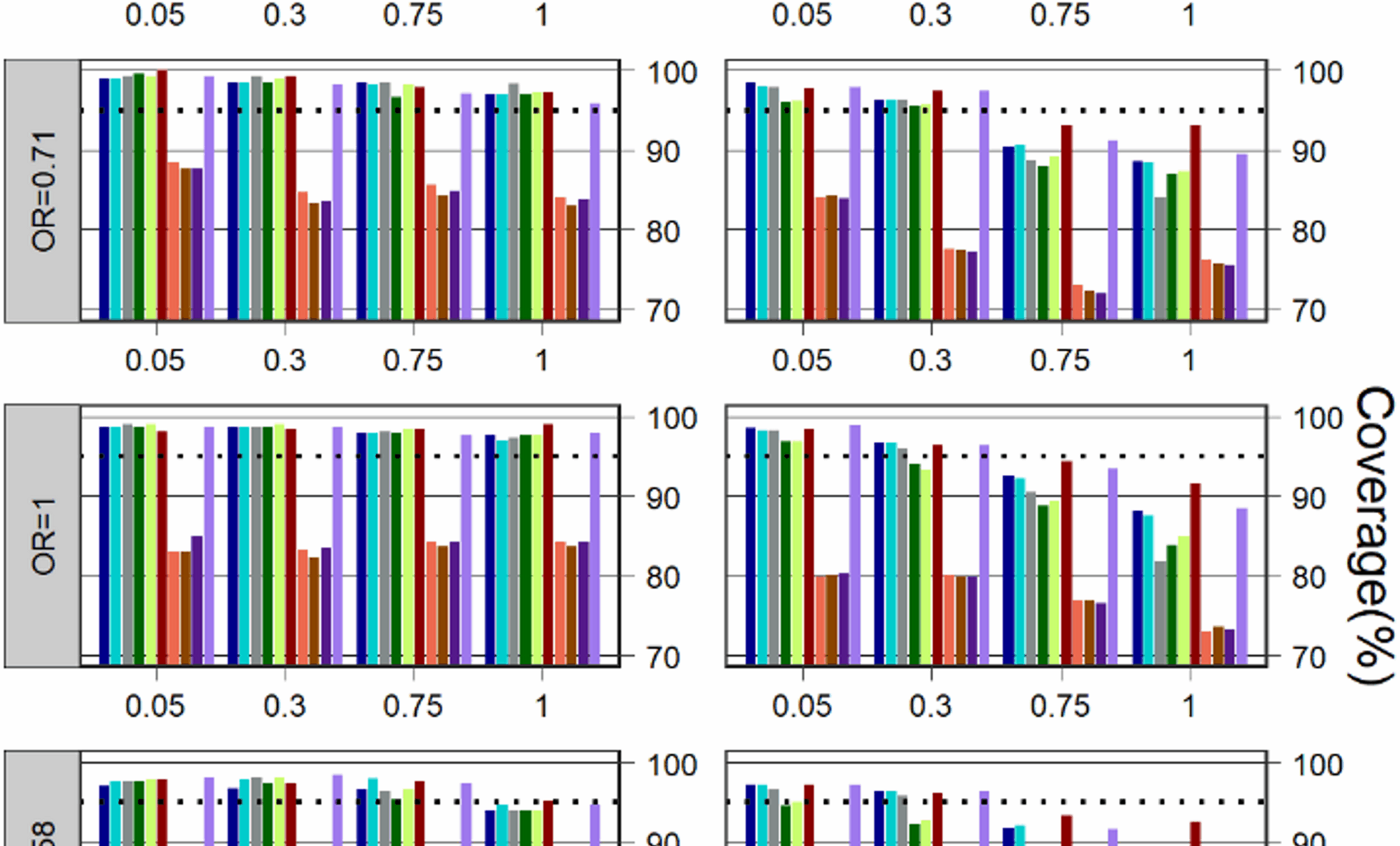
Coverage
Coverage for \(\:k=5\:\)is depicted in Fig. 1. Compared to the other models, GEE with different work correlation matrices often have a much lower coverage in all simulation scenarios. In most cases, regardless of treatment effect, control event rate, and heterogeneity, Betabin was usually among the models with the least affected, giving much better coverage than other models, followed by the Nchg.
Comparison of the different methods with respect to coverage for the simulated scenarios with \(\:k=5\). The dashed line depicts the nominal coverage level (95%)
When the heterogeneity was not large (=0.05 and 0.3), the performance of the methods based on coverage was consistently higher than the 95% level for all Bayesian and frequentist methods, but except for GLMM-A, GLMM-B and three GEE models in some cases where the control event rate was not very rare\(\:\:(\:{p}_{c}=0.05)\) and the treatment effect was also large (OR=1.58 and 2.86).
When the heterogeneity was large (=0.75 and 1), all Bayesian and frequentist methods (except for three GEEs) were able to maintain a coverage above or close to 95% in most cases for the scenarios where the control event rate was very rare (\(\:{p}_{c}=0.01\)); when the control event rate was not very rare (\(\:{p}_{c}=0.05\)), the Betabin also has a good coverage, Nchg, BNHM-1 and BNHM-2 have a similar coverage which was higher than GLMM-A, GLMM-B, and Beta-Hyperprior.
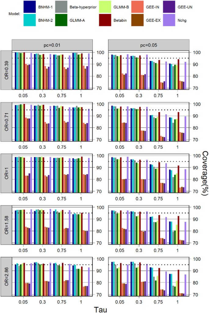
Bias
Median PB for \(\:k=5\) is presented in Fig. 2. The median PB of all methods is lower when the event rate is not very rare (\(\:{p}_{c}=0.05\)) compared to when it is (\(\:{p}_{c}=0.01\)). When the control event rate was not very rare \(\:\:(\:{p}_{c}=0.05)\), the Beta-Hyperprior has a relatively large median PB when the treatment effect was small (OR=0.39), the median PB is similar in magnitude for Betabin, three GEE models, and Nchg in most cases when the treatment effect was not small (OR = 0.71, 1, 1.58 and 2.86). When the control event rate was very rare \(\:\:(\:{p}_{c}=0.01)\) and the treatment effect was large (OR=1.58 and 2.28), the BNHM-2 has a relatively small median PB, but the Beta-Hyperprior has a relatively large median PB. When the control event rate was very rare \(\:\:(\:{p}_{c}=0.01)\), the BNHM-2 tended to have a smaller median PB when the treatment effect was null (OR=1) and not very small (OR = 0.71), whereas the GLMM-A had a smaller median PB when the treatment effect was very small (OR = 0.39).
Comparison of the different methods with respect to median percentage bias (PB) for the simulated scenarios with \(\:k=5\)
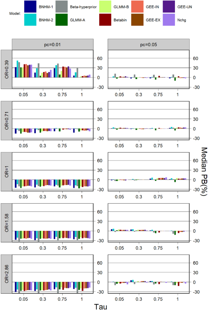
CI/CrI width
Median CI/CrI width for \(\:k=5\) is shown in Fig. 3. The median CI/CrI widths were generally large for a large treatment effect and a small control event rate. Across all simulation scenarios, GEEs with different working correlation matrices had the smallest median interval widths compared to other models, followed by Beta-hyperprior, while the BNHM-2 had the largest median interval widths in most scenarios. The median interval widths for the Betabin were larger than those for the three GEEs and the Beta-Hyperprior but smaller or comparable to those for the other models in most cases.
Comparison of the different methods with respect to median CI/CrI width for the simulated scenarios with \(\:k=5\)
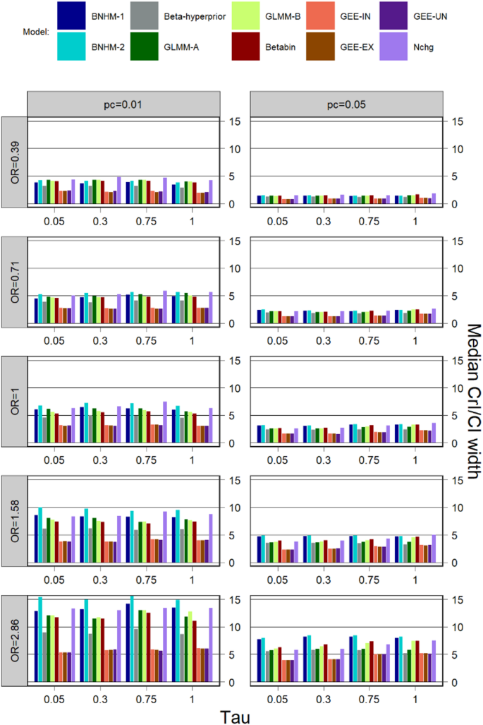
RMSE
The RMSE for \(\:k=5\) is exhibited in Fig. 4. For all models, the RMSE tends to be larger for a higher degree of heterogeneity and a larger treatment effect size. The RMSE for Nchg, three GEE models, BNHM-2, and GLMM-B is similar to each other, but is larger than that of the other models in most simulation scenarios. Beta-hyperprior consistently exhibited one of the lowest RMSE values across most scenarios. Under conditions of high heterogeneity (=0.75 and 1), the Betabin achieved a relatively low RMSE, though this remained higher than that of the Beta-hyperprior model and lower than those of the other models. In contrast, when heterogeneity was moderate or low (=0.05 and 0.3), the BNHM-1 demonstrated a small RMSE that was slightly higher than the Beta-Hyperprior, comparable to or lower than the Betabin, and consistently lower than those of the remaining models in most cases.
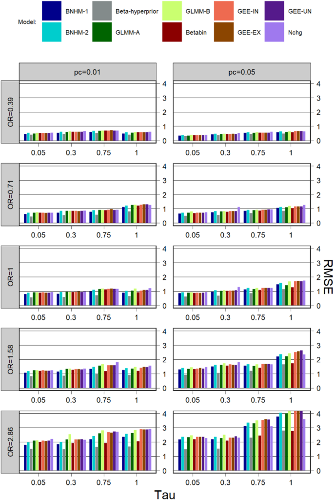
Comparison of the different methods with respect to RMSE for the simulated scenarios with \(\:k=5\)
Illustrative example
Model performance is further illustrated by applying the models presented above to two examples. The examples considered are come from two meta-analyses by Kishi et al. [46] that assessed the risk of mortality associated with long-acting injectable antipsychotics (LAI-AP) in patients with schizophrenia. These two meta-analyses pooled the data from RCTs comparing LAI-AP with placebo and oral antipsychotics (OAP). The analyses were based on the Peto method, a fixed-effects model. This section re-analyses the data and compares the results of the models described in Sect. 2. The data for both examples are illustrated in Tables 3 and 4.
Long-acting injectable antipsychotics versus placebos
The first example includes 18 RCTs comparing LAI-AP with placebos, of which eight were double-zero events studies and nine were single-zero events studies. A total of 13 events were reported in 5,919 randomized patients, and the incidence rate was about 0.2%. The sample size ratios ranged from 0.96 to 3.12. The results of the analyses are shown in the left panel of Fig. 5. Pooled OR estimates ranged from 0.26 (GLMM-A) to 0.72 (BNHM-2). All CIs/CrIs cover the null effect (OR = 1), which was very similar to the findings in the original analysis. Nchg yields the largest interval length, followed by GLMM-A and GLMM-B. The three GEE models produce narrower interval lengths, which is similar to the results of the simulation results summarized in Sect. 5.3. Among the three Bayesian approaches, the Beta-hyperprior had a narrower interval length, which is also similar to the simulation results.
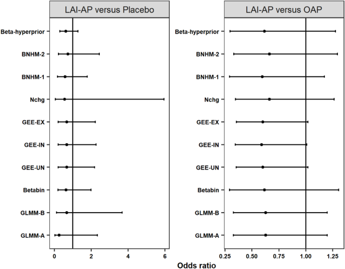
Estimated the risk of mortality associated with long-acting injectable antipsychotics among patients with schizophrenia using different methods. Left panel: long-acting injectable antipsychotics vs. placebos, right panel: long-acting injectable antipsychotics vs. oral antipsychotics
Long-acting injectable antipsychotics versus oral antipsychotics
The second analysis included 24 trials, of which seven were double-zero events studies and eight were single-zero events studies. A total of 39 events were reported, and the overall risk of death in both arms was about 0.5%. The sample size ratios ranged from 0.44 to 2.94. The results of the analyses are shown in the right panel of Fig. 5. The pooled OR estimates ranged from 0.59 (GEE-IN) to 0.66 (Nchg and BNHM-2). All CIs/CrIs covered the null effect (OR = 1), which was also very similar to the results of the original analysis. The CIs of the three GEE models have a narrower interval length than those obtained from the other models, which also is consistent with the simulation results.