The aim of developing the model is to simulate a refined petroleum products supply chain, comprehending the intricate dynamics of a multi-modal and multi-product network configuration and performance evaluation under diverse conditions. The proposed model serves as a representation of the designed supply chain network, utilizing parameters based on the average values obtained from the collected data. It serves as a fundamental framework for analyzing the intricate flows between entities and the inventory management at storage facilities. Employing Geographic Information System (GIS), the model utilizes the geographical coordinates of storage facilities and refineries to accurately estimate transport costs, particularly for road transportation networks. The initial deterministic model uses parameters in an environment having no disruptions, which will provide baseline values for material flow and total network costs. Later, the results from the initial model would be compared to models having disruptions in their supply chains.
Furthermore, another model is devised to account for disruptions in the supply chain, considering the impact of both demand and supply issues. This model optimizes the flow between entities, adapting to variations in the parameters associated with disruptions, which can be categorized as either random or predetermined. Based on the modelŌĆÖs results, potential mitigation strategies can be recommended to alleviate potential hindrances that might impede the smooth operation of the entire supply chain.
In the proposed MILP model, it is assumed that there exists a set R of refineries denoted by r, with respective supply capacities (Sr), a set D of distribution centers (depots) represented by d with product-specific capacities (Ud), and a set FS of demand nodes (fuel stations) designated as fs, with corresponding product demands denoted by p. The transport mode set T includes three modes (road, rail, and pipe). The complete notation utilized in the proposed model is delineated in Table┬Ā1.
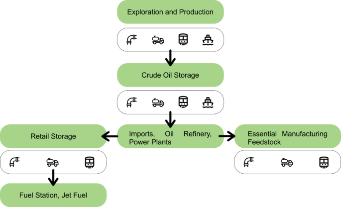
The supply chain proposed model includes the location of fuel storage facilities, refineries, and fuel stations along with their capacities. It also includes three modes of transport: flow of products from refineries to depots, transshipment of products between depots, and transport of products from depots to fuel stations. The model has the ability to choose from multiple modes of transportation to move products, provided if a certain mode is available. The following decisions need to be optimized considering the constraints of each entity in the supply chain:
Volume of products transported from refinery to depots.
Volume of products transported from ports to depots.
Volume of products transshipped between depots.
Volume of products transported from depots to fuel stations.
The objective function (1) minimizes the overall transport cost of the downstream oil supply chain from the refineries to the depots and from the depots to the fuel stations. The first term represents the combined cost of transport of products from refineries to depots, the second term represents the cost of transport of products from ports to depots while the third term is the transshipment cost between depots. The last term accounts for the cost to transport products from depots to fuel stations. Constraint (2) ensures that the demand for fuel at each fuel station is satisfied by the distribution centers. Constraint (3) limits the supply from the refineries to depot up to the refinery production limit. Constraint (4) ensures that the inflow of products from refineries, ports and other depots does not go beyond the storage capacity of products at each storage facility. Constraint (5) is the conservation of material at the storage facilities so that the flow of products to fuel station is not more than the flow of products into depots. Constraints (6) are non-negativity of the decision variables.
The mathematical formulation of the model is presented below.
Minimize:
$$\begin{gathered} \sum\limits_{{r\epsilon R}} {\sum\limits_{{d\epsilon D}} {\sum\limits_{{p\epsilon P}} {\sum\limits_{{t\epsilon T}} {{V_{r,d,p,t}} \cdot {C_{r,d,p,t}}} } } } \hfill \\ +\sum\limits_{{i\epsilon D}} {\sum\limits_{{d\epsilon D}} {\sum\limits_{{p\epsilon P}} {\sum\limits_{{t\epsilon T}} {{V_{i,d,p,t}} \cdot {C_{i,d,p,t}}} } } } \hfill \\ \quad +\sum\limits_{{d1\epsilon I}} {\sum\limits_{{d2\epsilon D}} {\sum\limits_{{p\epsilon P}} {\sum\limits_{{t\epsilon T}} {{V_{d1,d2,p,t}} \cdot {C_{d1,d2,p,t}}} } } } \hfill \\ \quad +\sum\limits_{{d\epsilon D}} {\sum\limits_{{fs\epsilon FS}} {\sum\limits_{{p\epsilon P}} {\sum\limits_{{t\epsilon T}} {{V_{d,fs,p,t}} \cdot {C_{fs,d,p,t}}} } } } \hfill \\ \end{gathered}$$
(1)
Subject to:
$$\sum\limits_{{d \in d}} {\sum\limits_{{fs \in FS}} {\sum\limits_{{p \in P}} {\sum\limits_{{t \in T}} {{V_{d,fs,p,t}} \cdot {D_{fs,p,}}} } } }$$
(2)
$$\sum\limits_{{r \in R}} {\sum\limits_{{d \in D}} {\sum\limits_{{p \in P}} {\sum\limits_{{t \in T}} {{V_{r,d,p,t}} \leqslant {S_{r,p}}\forall {\kern 1pt} r\epsilon R,p\epsilon P} } } }$$
(3)
$$\sum\limits_{{i \in I}} {\sum\limits_{{d \in D}} {\sum\limits_{{p \in P}} {\sum\limits_{{t \in T}} {{V_{i,d,p,t}}} } } } \leqslant {S_{i,p}}\forall {\kern 1pt} r\epsilon R,p\epsilon P$$
(4)
$$\begin{gathered} \sum\limits_{{r\epsilon R}} {\sum\limits_{{d\epsilon D}} {\sum\limits_{{p\epsilon P}} {\sum\limits_{{t\epsilon T}} {{V_{r,d,p,t}}+\sum\limits_{{i\epsilon I}} {\sum\limits_{{d\epsilon D}} {\sum\limits_{{p\epsilon P}} {\sum\limits_{{t\epsilon T}} {{V_{i,d,p,t}}} } } } } } } } \hfill \\ +\sum\limits_{{d1\epsilon D}} {\sum\limits_{{d2\epsilon D}} {\sum\limits_{{p\epsilon P}} {\sum\limits_{{t\epsilon T}} {{V_{d1,d2,p,t}} \leqslant {\kern 1pt} {\kern 1pt} {U_{d,p}}\forall d\epsilon D,p\epsilon P} } } } \hfill \\ \end{gathered}$$
(5)
$$\begin{gathered} \sum\limits_{{r\epsilon R}} {\sum\limits_{{d\epsilon D}} {\sum\limits_{{p\epsilon P}} {\sum\limits_{{t\epsilon T}} {{V_{r,d,p,t}}+\sum\limits_{{i\epsilon I}} {\sum\limits_{{d\epsilon D}} {\sum\limits_{{p\epsilon P}} {\sum\limits_{{t\epsilon T}} {{V_{i,d,p,t}}} } } } } } } } \hfill \\ +\sum\limits_{{d1\epsilon D}} {\sum\limits_{{d2\epsilon D}} {\sum\limits_{{p\epsilon P}} {\sum\limits_{{t\epsilon T}} {{V_{d1,d2,p,t}}=\sum\limits_{{d\epsilon D}} {\sum\limits_{{fs\epsilon FS}} {\sum\limits_{{p\epsilon P}} {\sum\limits_{{t\epsilon T}} {{V_{d,fs,p,t}}} } } } } } } } \hfill \\ \end{gathered}$$
(6)
Variables.
$$\begin{gathered} {V_{r,d,p,t}},\,{V_{i,d,p,t}},\,{V_{d1,d2,p,t}},\,{V_{d,fs,p,t}} \geqslant 0 \hfill \\ \forall r\epsilon R,\,i\epsilon I ,\,d,d1,d2\epsilon D,fs\epsilon FS,p\epsilon P,t\epsilon T \hfill \\ \end{gathered}$$
The deterministic model serves as the foundation for the subsequent Monte Carlo simulations. In the Monte Carlo simulation, the parameters of the transport cost per unit for each mode are adjusted, in addition to the supply of products from refineries and the demand of products at fuel stations. The network structure remains consistent during the Monte Carlo simulations, mirroring the deterministic case. The capacities of depots and the distances between all entities remain unchanged in both scenarios.
MONTE CARLO simulation based on the proposed model
The Monte Carlo simulation is a technique used for conducting sensitivity analysis, aimed at understanding how a model reacts to inputs generated in a stochastic manner. Typically, this process involves the random generation of inputs, or scenarios, followed by the execution of a simulation for each of these scenarios using a computerized model. The resulting outputs from these scenarios are evaluated and aggregated. Statistical analysis of these results provides key insights, including the mean value, output distribution, and the operational range of the model. Varying parameter values, encompassing fuel station demands, refinery supplies, and transport costs between entities, require the generation of distinct scenarios through Monte Carlo sampling. Each of these uncertain optimization models is then transformed into a deterministic optimization problem in its own right. The Python 3.11 programming language is employed to build the designed model, with PuLP 2.7 serving as the primary solver. To comprehensively explore the impacts of uncertainties on the model, several general cases for the scenarios are generated, including:
Disruption 1: High demand and low refinery output.
Disruption 2: Low demand and constant refinery output.
Disruption 3: Escalating transport costs per unit of fuel due to the cost-of-living crisis.
Disruption 4: The breakdown of the pipeline network, necessitating repair and leading to a shift in the transportation of oil.
The Monte Carlo simulation employs all these scenarios simultaneously to generate the flows of products between entities. The analysis involves assessing the simultaneous alterations to multiple parameters within the supply chain. Even though stochastic optimization and scenario analysis are widely used for uncertainty modelling, they face limitations in DOSCs. Stochastic optimization requires precise probability distributions, which are rarely available for disruptions such as refinery shutdowns, transport interruptions, or sudden demand shifts. Scenario analysis, on the other hand, evaluates only a limited number of predefined cases and cannot capture the full variability of real-world conditions. Monte Carlo simulation was therefore chosen for its ability to systematically sample from estimated ranges of uncertain parameters and generate a large number of possible realizations. By repeatedly solving the MILP model under these realizations, the approach provides not only expected costs but also the variance and risk profile of the supply chain. This makes Monte Carlo particularly valuable for assessing resilience, as it quantifies how disruptions of different magnitudes and frequencies influence flows and costs across the network.
Parameter setup
To assess the efficacy of the formulated model, a practical case study of a downstream petroleum supply chain for a company is selected. The countryŌĆÖs population distribution indicates that the highest demand for transportation fuel lies in the northeastern province of Punjab. Sindh, particularly Karachi, serves as the nationŌĆÖs most significant industrial center and accounts for the second-highest fuel consumption. On the other hand, the demand for fuel is relatively low in KPK and Baluchistan due to limited industrialization and a scattered population. However, since the majority of refineries and import terminals are situated in the southern part of the country, transportation of fuel to the north is necessary to meet the demand.
For the initial deterministic model, the parameters are configured based on the companyŌĆÖs daily refined fuel sales nationwide, alongside the average daily refinery output. The refineries production capacities vary between 0.8┬Āmillion to 3.0┬Āmillion liters per day; however, an average output is utilized for the initial model. The storage capacity of depots also varies, with the largest being close to 160┬Āmillion liters while the smallest is around 0.2┬Āmillion liters. The pipeline and railway networks are obtained from government reports, while the road network is established using GIS data. In this deterministic model, 3,500 fuel stations are considered, representing approximately 36% of the total operational fuel stations in the country, without any provincial divisions due to inter-provincial sale instances. The country is equipped with 5 refineries, each contributing to the supply of products according to their capacities. Additionally, 25 storage facilities are distributed across the nation, each with specific product capacities based on actual distribution requirements. No disruptions or capacity constraints are incorporated in this model, allowing for the verification of a fully operational model with all associated constraints.
The MILP model is designed to ascertain the minimized cost of transporting refined fuel products in accordance with the demands of fuel stations. The primary decision variables include the flow of products between entities via various transportation modes. Modeling for random disruptions involves the alteration of parameters through scenario generation, adhering to standardized deviation criteria.