Continuous design and reprogramming of Totimorphic structures for space applications

In the following, we describe the mathematical models referenced in the main text, including mathematical proofs. These are just one particular realisation of an analytical Totimorphic model, and the introduced framework can be extended to other Totimorphic structures in a straightforward way. Implementations of the models in Python are available on Github 26. Simulation details are provided at the end of this section.

Notation

We first introduce the notation used in the following sections. Polar vectors are denoted by:

For proofs, we will be using the identity:

We also introduce theoperator \(E(\cdot ):{{\rm{{\mathbb{R}}}}}^{2}\to {\rm{{\mathbb{R}}}}\) that returns the angles α required to represent a vector r in polar coordinates, given by:

Rotation matrices in three-dimensional Euclidean space are given by:

Similarly, we denote the standard polar vector in three dimensions by:

To gain the angles for representing a general vector r in these coordinates, we introduce \(\Xi (\cdot ):{{\rm{{\mathbb{R}}}}}^{3}\to {{\rm{{\mathbb{R}}}}}^{2}\) given by:

We further use the following polar representation:

with

To gain the angles for representing a general vector r in these coordinates, we introduce \({\mathcal{E}}(\cdot ):{{\rm{{\mathbb{R}}}}}^{3}\to {{\rm{{\mathbb{R}}}}}^{2}\) given by:

For proofs, the following identity is used:

Totimorphic lattices in two dimensions

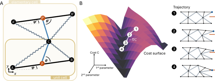
In the following, we drop the index ij (cell at row i and column j) for clarity. However, all vectors are always given per elementary cell (see main text). An elementary cell is constructed from two unit cells which are connected at their levers. An elementary cell in the Totimorphic lattice is parameterised by \(({\boldsymbol{o}},\varphi ,\theta ,{\varphi }^{{\prime} },{\theta }^{{\prime} })\), where o is the location of point A, φ is the angle with the x-axis of the lower beam, and θ is the angle of the lower lever with respect to the lower beam. Primed variables represent the same quantities, but for the upper half of the elementary cell (i.e., the upper beam and lever).

The points of the lower unit cell are given by:

The points of the upper unit cell are given by:

For the upper triangle, we recover \({\varphi }^{{\prime} }\) via

and \({\theta }^{{\prime} }\) through

with \({\varphi }^{{\prime} }\) given by Eq. (25).

To check for overlapping springs in the elementary cell, representing a state in which the cell physically breaks, we introduce the following angles per elementary cell:

αL is the angle of the bottom left spring (connecting points A and C) with the x-axis, while αR is the angle of the bottom right spring (connecting points B and C). Primed angles indicate the same for the top unit cell. Angles are measured with respect to the x-axis going through point C, hence in the flat configuration, top angles are negative and bottom angles are positive.

Connecting elementary cells in two dimensions

The first elementary cell (i = 0, j = 0) can be constructed freely, as there are no other cells to connect it to. Adding more unit cells horizontally (i = 0, j > 0) is done iteratively as follows. First, we enforce the constraint of connecting the two elementary cells:

Then we have to obtain the point \(\rm{P}^{\prime}\) of our new elementary cell, which has to satisfy the beam and lever constraints. In the following, all points are in the same elementary cell (0j), and thus we drop the indices for convenience. The condition for the existence of \({{\boldsymbol{r}}}^{{{\rm{P}}}^{{\prime} }}\) is that lever and beam with fixed length have to connect to it from point \({\rm{A}}^{\prime}\) (given by the first elementary cell) and point C:

Introducing \({{\boldsymbol{s}}}^{-}={{\boldsymbol{r}}}^{{{\rm{A}}}^{{\prime} }}-{{\boldsymbol{r}}}^{{\rm{C}}}\), \({{\boldsymbol{s}}}^{+}={{\boldsymbol{r}}}^{{{\rm{A}}}^{{{\prime} }}}+{{\boldsymbol{r}}}^{{\rm{C}}}\) and \(\delta =\frac{1}{2}(\parallel {{\boldsymbol{r}}}^{{{\rm{A}}}^{{\prime} }}{\parallel }^{2}-\parallel {{\boldsymbol{r}}}^{{\rm{C}}}{\parallel }^{2})\), we get

Proof: derivation of expression for \({{\rm{P}}}^{{\prime} }\)

In the following, we do not write the indices ij explicitly to simplify the notation.

First, we start from the condition that \({{\rm{P}}}^{{\prime} }\) has to be chosen such that the resulting beam (connecting \({{\rm{A}}}^{{\prime} }\) and \({{\rm{P}}}^{{\prime} }\)) and lever (connecting C and \({{\rm{P}}}^{{\prime} }\)) have the desired length:

Expanding both expressions, subtracting Eq. (40) from Eq. (39) and dividing the resulting equation by 2, we obtain:

Using the notation \({{\boldsymbol{s}}}^{-}={{\boldsymbol{r}}}^{{{\rm{A}}}^{{\prime} }}-{{\boldsymbol{r}}}^{{\rm{C}}}\), \({{\boldsymbol{s}}}^{+}={{\boldsymbol{r}}}^{{{\rm{A}}}^{{\prime} }}+{{\boldsymbol{r}}}^{{\rm{C}}}\) and \(\delta =\frac{1}{2}(\parallel {{\boldsymbol{r}}}^{{{\rm{A}}}^{{\prime} }}{\parallel }^{2}-\parallel {{\boldsymbol{r}}}^{{\rm{C}}}{\parallel }^{2})\) this yields Eq. (37). To obtain Eq. (38), we first insert Eq. (37) into Eq. (40) and rewrite it to match the form of a quadratic equation:

Writing out all terms in the numerator of p (denoted by pn), it can be simplified to

Using the two identities:

we arrive at

and thus

For q, we first note (using binomial formulas) that

Using \({\delta }^{2}-2\delta {r}_{x}^{{\rm{C}}}{s}_{x}^{-}+{({r}_{x}^{{\rm{C}}}{s}_{x}^{-})}^{2}={(\delta -{r}_{x}^{{\rm{C}}}{s}_{x}^{-})}^{2}\) as well as \({(\frac{p}{2})}^{2}=\frac{1}{4}{({r}_{y}^{{{\rm{A}}}^{{\prime} }}+{r}_{y}^{{\rm{C}}})}^{2}[{({r}_{x}^{{{\rm{A}}}^{{\prime} }}-{r}_{x}^{{\rm{C}}})}^{2}+{({r}_{y}^{{{\rm{A}}}^{{\prime} }}-{r}_{y}^{{\rm{C}}})}^{2}]\), we can then calculate the remaining term \({(\frac{p}{2})}^{2}-q\) required for solving Eq. (42). First. we only look at all terms in \({(\frac{p}{2})}^{2}-q\) not containing lb. The numerator of this term is given by:

The terms containing lb simplify to \(\frac{{l}_{b}^{2}{({s}_{x}^{-})}^{2}}{4\parallel {{\boldsymbol{s}}}^{-}{\parallel }^{2}}\). Using the previous results, we arrive at:

Finally, putting everything together, we can solve Eq. (42) using the p-q formula and by inputting the results for p and \({(\frac{p}{2})}^{2}-q\):

\(\frac{1}{2}{{\boldsymbol{s}}}^{+}\) is the mid-point of the spring connecting point C and \({\rm{A}}^{\prime}\). Hence, \({s}_{y}^{+}\) is its y coordinate (or height). If point \({\rm{A}}^{\prime}\) is left of point C, as e.g. in the initial flat configuration, point \({\rm{P}}^{\prime}\) has to be above this spring; meaning that its y coordinate has to be larger than \({s}_{y}^{+}\). Since \({s}_{x}^{-}\) is negative in this scenario, the minus sign has to be chosen to get the correct solution. Similarly, if we pivot the unit cell such that \({s}_{x}^{-}=0\), i.e., \(\rm{A}^{\prime}\) and C lie above each other, we have that \({r}_{y}^{{{\rm{P}}}^{{\prime} }}=\frac{1}{2}{s}_{y}^{+}\). Pivoting further, \({\rm{P}}^{\prime}\) is situated below the spring (although it never swapped sides), as given by Eq. (38). Thus, when starting from the flat hour-glass motive, we have to choose the negative sign to get the correct solution for \({\rm{P}^{\prime}}\).

Conditions for intact elementary cells in two dimensions

The criteria for being intact are the same for every unit cell (ij), therefore indices are dropped again in the following to ease notation. An elementary cell is considered intact if the following conditions are met:

The first condition means that springs cannot be stretched further than the beam length (for a solution of \({{\boldsymbol{r}}}^{{{\rm{P}}}^{{\prime} }}\) to exist, Eq. (38) has to be a real number, meaning that the argument of the square root has to be larger or equal to zero. This immediately yields Eq. (55)). The second (third) conditions check whether the left (right) bottom and top springs cross.

To avoid overstretched springs, we correct θ by constraining its range. The limits of this interval are obtained by the criterion for the existence of real-valued solutions of Eq. (38) (the term below the root has to be ≥ 0):

with \({\boldsymbol{k}}={{\boldsymbol{r}}}^{{{\rm{A}}}^{{\prime} }}-{{\boldsymbol{r}}}^{{\rm{A}}}-\frac{{l}_{{\rm{b}}}}{2}{{\boldsymbol{e}}}^{\varphi }\), \(\Phi =E({\boldsymbol{k}})\), \({\varDelta} ={\varPhi}-{\varphi}\), and \(C=\frac{\parallel {\boldsymbol{k}}\parallel }{{l}_{b}}-\frac{3}{4}\frac{{l}_{b}}{\parallel {\boldsymbol{k}}\parallel }\).

If the interval for θ is empty, it is impossible to add a new elementary cell without changing the configuration of previous cells in the structure. These conditions are checked for each unit cell separately while constructing it.

Proof: deriving allowed range of θ

First, we write out rC in s−:

with \({\boldsymbol{k}}={{\boldsymbol{r}}}^{{{\rm{A}}}^{{\prime} }}-{{\boldsymbol{r}}}^{\rm{A}}-\frac{{l}_{{\rm{b}}}}{2}{{\boldsymbol{e}}}^{\varphi }\). This way, we split up s− into two terms – one depending on θ, and one that is independent of θ, summarising the geometric constraints introduced by the previous unit cell. By representing k in polar coordinates, we arrive at

with \(\Phi =E({\boldsymbol{k}})\), which simplifies the following derivation of the range of θ. To guarantee that a solution for point \(\rm{P}^{{\prime} }\) exists, Eq. (55) has to be fulfilled. By squaring Eq. (55) and using Eq. (62), we get

where we used Eq. (6) and introduced \({\varDelta} = {\varPhi} – {\varphi}\), and \(C=\frac{\parallel {\boldsymbol{k}}\parallel }{{l}_{{\rm{b}}}}-\frac{3}{4}\frac{{l}_{{\rm{b}}}}{\parallel {\boldsymbol{k}}\parallel }\). From this, we can invert the cosine function to get

from which we get the upper (choosing −) and lower (choosing +) bound of θ shown in Eq. (58).

Building a two-dimensional Totimorphic structure

For i > 0 and j = 0, one sets \(\varphi_{i0} ={\varphi }^{{\prime} }_{i-1,0}\), \({{\boldsymbol{r}}}_{i,0}^{{\rm{A}}}={{\boldsymbol{r}}}_{i-1,0}^{{{\rm{A}}}^{{\prime} }}\), and calculates all points as for the first elementary cell (i = 0, j = 0). In all remaining cases, we set \(\varphi_{ij} ={\varphi }^{{\prime} }_{i-1,j}\), \({{\boldsymbol{r}}}_{i,j}^{{\rm{A}}}={{\boldsymbol{r}}}_{i,j-1}^{{\rm{B}}}\), \({{\boldsymbol{r}}}_{ij}^{{{\rm{A}}}^{{\prime} }}={{\boldsymbol{r}}}_{i,j-1}^{{{\rm{B}}}^{{\prime} }}\), and calculate the remaining points by solving for \(\rm{P}^{{\prime} }\).

Depending on where in the lattice an elementary cell is positioned, it is characterised by the following parameters:

1.

i = 0, j = 0: \(({{\boldsymbol{o}}}_{00},\varphi_{00} ,\theta_{00} ,{\varphi }^{{\prime} }_{00},{\theta }^{{\prime} }_{00})\),

2.

i = 0, j > 0: (\(\varphi_{0j}\), \(\theta_{0j}\)),

3.

i > 0, j = 0: \((\theta_{i0} ,{\varphi }^{{\prime} }_{i0},{\theta }^{{\prime} }_{i0})\),

4.

else: (\(\theta_{ij}\)).

To initialise the lattice as a flat surface, beam angles \({\varphi}_{ij}\) and \({\varphi }^{{\prime} }_{ij}\) have to be set to 0 and lever angles \(\theta_{ij}\) and \({\theta }^{{\prime} }_{ij}\) to \(\frac{\pi }{2}\,\,\forall i,j\).

Totimorphic lattices in three dimensions

As in the two-dimensional case, each elementary cell is characterised by the angles of the beams and levers, \(({\boldsymbol{o}},{\varphi }_{y},{\varphi }_{z},{\theta }_{x},{\theta }_{z},{\varphi }_{y}^{{\prime} },{\varphi }_{z}^{{\prime} },{\theta }_{x}^{{\prime} },{\theta }_{z}^{{\prime} })\).

The points of the lower unit cell are given by:

Here, the beam is described by its rotation in the x–y plane (given by φz, which corresponds to φ in the two-dimensional case) and a rotation in x–z plane (a tilting of the unit cell given by φy). The orientation of the lever is obtained by a sequence of rotations: first, we rotate the x-direction unit vector 1x by θz (in the two-dimensional case, we called this θ), then tilt it in the y-z plane by θx, and then apply the same transformation (two rotations) used to gain the beam vector from the unit vector. We choose this parametrisation so that the angles of the lever are again defined with respect to the orientation of the beam, as in the two-dimensional case.

The points of the upper unit cell are defined similarly:

Connecting elementary cells in three dimensions

Again, the first elementary cell (i = 0, j = 0) is unconstrained and can be constructed freely. Without loss of generality, we initialise lattices lying in the x–z plane. Adding more unit cells horizontally (i = 0, j > 0) is done iteratively as follows. First, we enforce the constraint of connecting the two elementary cells:

In the following, all points are in the same elementary cell (0j), and thus we drop the indices for convenience. As in the two-dimensional case, we look again for a consistent solution for \({{\boldsymbol{r}}}^{{{\rm{P}}}^{{\prime} }}\). The vector representing the upper beam is given by lb ⋅ ξϕ,Θ (the traditional angles are recovered via \(({\varphi }_{y},{\varphi }_{z})={\mathcal{E}}({{\boldsymbol{\xi }}}^{\phi ,\Theta })\). The lever is then given by the vector

For \({\rm{P}}^{\prime}\) to exist, the lever has to have the correct length:

From this, we obtain a solution for \(\phi\) and \(\varTheta\), with \(\phi\) being completely determined by \(\varTheta\). Additionally, as in the two-dimensional case, we gain valid intervals for both \(\varTheta\) as well as \(\theta_z\).

The remaining points are then given by:

Proof: deriving expressions for ϕ and Θ

Expanding Eq. (79), we get

Writing s− in spherical coordinates with \((\alpha ,\beta )=\Xi ({{\boldsymbol{s}}}^{-})\), this becomes

or, using Eq. (16),

from which we get the solution for \(\phi\) depending on \(\varTheta\):

The arccos can have two signs, so as in the two-dimensional case, two solutions exist. We found that when starting with the flat surface configuration, a minus sign has to be chosen. However, different from the two-dimensional case, the alternative solution (+ instead of −) also represents a valid Totimorphic configuration, although the two obtained configurations are far apart. In the case \(\sin \beta =0\), \(\phi\) can be freely chosen and \(\varTheta\) has a unique solution \(\Theta =\arccos \left(-\frac{\parallel {{\boldsymbol{s}}}^{-}\parallel }{{l}_{{\rm{b}}}\cos \beta }\right)\). In this case, the spring vector s− is parallel to the z-axis. Any solution given by \(\varTheta\) will now form a triangle, from \({{\rm{A}}}^{{\prime} }\) to \({{\rm{P}}}^{{\prime} }\), from \({{\rm{P}}}^{{\prime} }\) to C, and from C back to \({{\rm{A}}}^{{\prime} }\) (which is parallel to the z-axis). Changing ϕ will now rotate this triangle around the z-axis without distorting it, hence there is an infinite amount of valid configurations that lie on a circle around the z-axis.

If \(\sin \beta \ne 0\) (i.e., β ≠ 0, which is almost always the case as β = 0 is a singular point), \({\mathcal{C}}\) has to be in the allowed range of \(\arccos\):

Note that in spherical coordinates, β ∈ [0, π], and hence we always have \(\sin \beta \ge 0\) (and similarly \(\sin \Theta \ge 0\)). From \({\mathcal{C}}\ge -1\), we get

and, by using \(\sin (2\pi -\beta )=-\sin \beta\), \(\cos (2\pi -\beta )=\cos \beta\), and \(\cos (2\pi -\beta )\cos \Theta +\sin (2\pi -\beta )\sin \Theta =\cos (2\pi -\beta -\Theta )\),

which yields

This range is valid when \({\mathcal{C}}\le 0\). If \({\mathcal{C}}\ge 0\), we have to guarantee that \({\mathcal{C}}\le 1\), which results in

Proof: deriving allowed range of θ
z

Finally, we can calculate an allowed range for θz (as in the 2D case). This can be derived by requiring that the \(\arccos\) in Eq. (89) and (90) has a valid solution, i.e.,

First, we rewrite s− by expanding it:

To isolate θz, we rotate s− by Rx(− θx)Rz(− φz)Ry(− φy), which gives us

with \({\boldsymbol{k}}={R}_{x}(-{\theta }_{x}){R}_{z}(-{\varphi }_{z}){R}_{y}(-{\varphi }_{y})\cdot ({{\boldsymbol{r}}}^{{{\rm{A}}}^{{\prime} }}-{{\boldsymbol{r}}}^{{\rm{P}}})\). Since rotations leave the length of a vector unchanged, we can thus rewrite condition Eq. (91) as

We solve this the same way as in Eq. (58), resulting in

with \(({\theta }_{k},{\phi }_{k})=\Xi ({\boldsymbol{k}})\). Using \({{\boldsymbol{\xi }}}^{{\theta }_{k},{\phi }_{k}}\cdot {{\boldsymbol{\xi }}}^{{\theta }_{z},\frac{\pi }{2}}=\sin {\phi }_{k}\cdot \cos ({\theta }_{k}-{\theta }_{z})\), we get

from which the final interval is derived

Building a three-dimensional Totimorphic structure

For i > 0 and j = 0, one sets \({\varphi }_{z;{i}{0}}={{\varphi }^{{\prime}}}_{z;{i-1},{0}}\), \({\varphi }_{y;i0}={{\varphi }^{{\prime} }}_{y;i-1,0}\), \({\boldsymbol{r}}_{i,0}^{\rm{A}}={{\boldsymbol{r}}}_{i-1,0}^{{\rm{A}}^{\prime}}\), and calculates all points as for the first unit cell (i = 0, j = 0). In all remaining cases, we set \({\varphi }_{z;i0}={{\varphi }^{{\prime} }}_{z;i-1,0}\), \({\varphi }_{y;i0}={{\varphi }^{{\prime} }}_{y;i-1,0}\), \({{\boldsymbol{r}}}_{i,j}^{{\rm{A}}}={{\boldsymbol{r}}}_{i,j-1}^{{\rm{B}}}\), \({{\boldsymbol{r}}}_{ij}^{{{\rm{A}}}^{{\prime} }}={{\boldsymbol{r}}}_{i,j-1}^{{{\rm{B}}}^{{\prime} }}\), and calculate the remaining points by solving for ϕ and Θ.

Depending on where in the lattice an elementary cell is positioned, it is characterised by the following parameters (we drop indices here for clarity, but all parameters are different):

1.

i = 0, j = 0: \(({\boldsymbol{o}},{\varphi }_{y},{\varphi }_{z},{\theta }_{x},{\theta }_{z},{\varphi }_{y}^{{\prime} },{\varphi }_{z}^{{\prime} },{\theta }_{x}^{{\prime} },{\theta }_{z}^{{\prime} })\)

2.

i = 0, j > 0: (φy, φz, θx, θz, Θ)

3.

i > 0, j = 0:\(({\theta }_{x},{\theta }_{z},{\varphi }_{y}^{{\prime} },{\varphi }_{z}^{{\prime} },{\theta }_{x}^{{\prime} },{\theta }_{z}^{{\prime} })\)

4.

else: (θx, θz, Θ)

To initialise the lattice as a flat surface in x–z plane, beam angles φz;ij and \({{\varphi }^{{\prime} }}_{z;ij}\) have to be set to \(\frac{\pi }{2}\) and all remaining angles to 0.

Methodology for the first proof of concept: direct stiffness method

The fundamental building block of the direct stiffness method is rod or beam-like elements characterised by the coordinates of its two ending points \(i,j\in {\rm{{\mathbb{N}}}}\), i.e., (xi, yi) and (xj, yj). Applying forces (Fi, Fj) to the two ending points of the element results in a deformation of the element; or more specifically, a displacement of the ending points (ui, uj), which is calculated from the stiffness equation (a generalisation of Hook’s law):

with Kij being the stiffness matrix, and \({{\boldsymbol{u}}}_{i}=({u}_{i}^{x},{u}_{i}^{y},{u}_{i}^{\varphi })\) being the resulting displacements due to external forces and moments \({{\boldsymbol{F}}}_{i}=({F}_{i}^{x},{F}_{i}^{y},{M}_{i}^{\varphi })\). φ characterises the resulting bending of beam elements. Thus, the updated equilibrium state of the beam after applying forces is given by \(({x}_{i}+{u}_{i}^{x},{y}_{i}+{u}_{i}^{y})\) and \(({x}_{j}+{u}_{j}^{x},{y}_{j}+{u}_{j}^{y})\). Repeating this process by recalculating the stiffness matrix using the updated coordinates and solving Eq. (98) anew, deformations due to larger forces can be obtained.

Generalised Euler-Bernoulli beam elements

In this work, we use generalised Euler-Bernoulli beam elements to model the beams and levers in a Totimorphic lattice. The stiffness matrix Kij of the generalised beam element is obtained by combining the stiffness matrices of rod elements, i.e., elements that behave like springs,

and Euler-Bernoulli beam elements that model bending27

resulting in

Here, Lij is the length of the beam, and sij and cij are the sine and cosine of the angle ϑij of the beam with respect to the x-axis:

Eij, Aij, and Iij are the elements Young’s modulus, cross-sectional area, and second moment of area, respectively. For simplicity, we choose a uniform lattice with Eij = E, Iij = I, and Aij = A.

Compression experiment

The global stiffness matrix G of a whole lattice structure is obtained by adding up the stiffness matrices of the individual beams and levers accordingly. The stiffness equation for the whole structure then takes the same form as the one for individual elements, but it contains all lattice point coordinates (ending points of Totimorphic beams or levers, i.e., points A, \(\rm{A}^{\prime}\), B, \(\rm{B}^{\prime}\), P, \(\rm{P}^{\prime}\),C and of each elementary cell):

To implement the compression experiment, we first set the displacement of points that are part of the top surface of the lattice to a small non-zero value. As boundary conditions, we set the displacement of all points in the bottom surface to zero (otherwise, the lattice would start moving downwards). Using Eq. (105) (i.e. matrix multiplication), we calculate the resulting forces for all other points due to these forced displacements—from which we subsequently calculate the resulting displacements of all remaining points in the lattice that are not part of the top or bottom surface by solving a system of linear equations. We repeat this process several times (with updated global stiffness matrix G) to obtain macroscopic deformations. For a detailed description, see ref. 20.

Poisson’s ratio

Assume we do k iterations in the compression experiment, i.e., we solve Eq. (105) k times in sequence, and in each iteration we displace the top lattice points by ϵk. After each iteration, we collect the displacement in x-direction of the outer left and outer right points of the lattice, calculate the mean displacement over these points, and then obtain the average change in width of the lattice by taking the difference:

where \({\mathcal{L}}{\mathcal{S}}\) (\({\mathcal{R}}{\mathcal{S}}\)) is a set containing the indices of the points on the left (right) surface of the lattice. The outer points are given(left side) by points A’ and \({{\rm{A}}}^{{\prime} }\) of the first (i.e. outer left) column of elementary cells in the lattice, and (right side) by the points B and \({{\rm{B}}}^{{\prime} }\) of the last column (i.e. outer right) of elementary cells. \(| {\mathcal{R}}{\mathcal{S}}|\) denotes the number of elements in \({\mathcal{R}}{\mathcal{S}}\). The Poisson’s ratio is obtained using linear regression

The deformation in vertical direction is imposed on the top points, i.e., \({{\rm{A}}}^{{\prime} }\) and \({{\rm{B}}}^{{\prime} }\) of all elementary cells in the top roow, while the bottom points (A and B of all elementary cells in the bottom row) are kept static.

Alternative ways of calculating the Poisson ratio are possible, e.g., by imposing target displacements for the outer nodes in the cost function (e.g., no displacement to reach a Poisson ratio of 0, as done in ref. 20, Fig. 6C). Furthermore, to enforce symmetric behaviour during compression, additional terms can be added to the cost function that punish asymmetric deformations under load.

Methodology for the second proof of concept: ray-based optics

In the telescope mirror application, for simplicity, we only simulate light rays getting reflected at the mid-point (i.e. the mid-point of the lever) of each unit cell. Thus, each unit cell acts as a tiny mirror reflecting a single beam of light. We assume light coming from a source that is far away, such that the light rays hitting the different mirror elements are parallel to each other.

Reflections

To calculate the light reflection, we have to know the orientation of the surface of reflection, which is given by the normal vector of each unit cell. For a single elementary cell, the normal vectors of its two unit cells are

where ∥ ⋅ ∥2 is the Euclidean norm, × the vector cross product, and the primed vector denotes the top unit cell. The mid-points of the levers where the light is reflected are

Given a light ray with incidence direction I (∥I∥2 = 1), the directions of the reflected light lij coming from elementary cell (ij) are given by

where ⋅ is the vector dot product.

Smallest distance to the target focal point

Given a target focal point ftgt, we calculate the closest point cij (\({{\boldsymbol{c}}}_{ij}^{{\prime} }\)) along the reflected ray to it as follows:

We then calculate the following cost function

and optimise the Totimorphic lattice by updating its parameters via gradient descent, \(-{\nabla }_{{\mathcal{P}}}C({\mathcal{P}},{{\boldsymbol{f}}}^{{\rm{t}}{\rm{g}}{\rm{t}}})\).

Damaging mirror elements

To emulate a damaged mirror element, we add a random perturbation to the direction of the reflected light. For instance, assuming the bottom unit cell of element (ij) was damaged, we first sample a random deflection \({{\boldsymbol{l}}}_{\sigma } \sim {\mathcal{N}}(0,{\sigma }^{2})\) from a Gaussian distribution (with mean 0 and variance σ2) and always add it to the reflected light direction:

For a single experiment, lσ is only sampled once and kept constant afterwards

Imaging

For imaging, we assume a picture of Pluto with the same diameter and distance as the Moon (radius of rm ≈ 1700 ⋅ 103 m and angular radius of ϕm ≈ 0.25∘) has been placed at the same distance as the Moon (given by \({d}_{m}={r}_{m}/\arctan {\phi }_{m}\)).

For a 2S × 2S pixel image of Pluto, the light ray coming from the pixel in row i and column j (counted from the bottom left corner of the image) has the non-normalised incidence vector

and the normalised one \({{\boldsymbol{I}}}_{ij}=\frac{{\widetilde{{\boldsymbol{I}}}}_{ij}}{\parallel {\widetilde{{\boldsymbol{I}}}}_{ij}{\parallel }_{2}}\). To get an image, we reflect the light rays coming from every pixel in the image at every Totimorphic mirror element and check where on the imaging plane the reflections hit. For instance, if the imaging plane is at distance dz, the light ray Ikl reflected at the bottom unit cell of element (ij) hits the plane at mij + λ ⋅ lij with \(\lambda =({d}_{z}-{m}_{ij,z})/{l}_{ij,z}\) (z denoting the z-component of the vectors). For visualisation, we plot all reflected points in a two-dimensional image with point size s = 2 (in matplotlib) and an alpha (opacity) of 0.05, so that colours merge when multiple points overlap.

Simulation details: inverse lattice design

For the results shown in Fig. 4, during inverse design, we used a total external displacement of 0.2 applied through 5 iterations of the compression experiment. The cost function was optimised using the Adam optimiser (learning rate of 5 ⋅ 10−3 and no weight decay). To ensure that the top layer of nodes in the lattice remains flat, we added regularisation terms to the cost function, i.e., L1 loss terms that encode the difference in y-coordinate for points in the top layer. The training setup for negative and positive target Poisson’s ratio was identical apart from initialisation. For the positive target, we perturbed the initial configuration before training by adding Gaussian noise to each lattice parameter; drawn randomly from \({\mathcal{N}}(\mu =0,\sigma =1{0}^{-2})\). To visualise the final lattice designs in Fig. 4 and Fig. S1, we used a total external displacement of 0.325 and 0.5, respectively, applied over 30 iterations instead. For the results shown in Fig. S1, we trained with a target Poisson’s ratio of νtgt = − 2.

Simulation details: Totimorphic telescope

We trained the lattice only on the task of focusing light from one direction (i.e., orthogonal to the initially flat mirror surface) into a single point (focal point on the central axis orthogonal to the initially flat mirror surface) located at \((\frac{D}{2},\frac{D}{2},n\cdot D\), where D = 6m is the diameter (or side length) of the Totimorphic lattice and n an integer that we choose during training (e.g., we start with 20). For training configurations at different focal lengths, we used the Adam optimiser with a learning rate of 10−3, which is reduced to 10−4 if the root mean square loss goes below 5 ⋅ 10−3. We further always add a second cost term (with prefactor of 0.1) which has the objective of keeping the central node (point \({B}^{{\prime} }\) of the central elementary cell) of the lattice fixed in space. This is done to avoid that the lattice moves around in space during optimisation.

For the circle experiment in Fig. 7, we guide the focal point in a circle with radius \(\frac{D}{2}\) around its initial location (still with a focal length of 20D. We use the following learning rate scheme for this: starting with a learning rate of 10−3, we reduce it to 10−4 and 10−5 when the root mean square loss goes below 5 ⋅ 10−2 and 5 ⋅ 10−3, respectively.

For the self-repair experiments in Fig. 7, we select the damaged unit cell randomly and draw the deflection due to damaging randomly from \({\mathcal{N}}(0,5\cdot 1{0}^{-4})\). During training, we start with a learning rate of 10−4, which is reduced to 10−5 of the root mean square loss goes below 5 ⋅ 10−3.