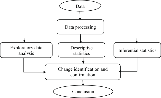
Results of the exploratory data analysis
The lake annual mean water level for the regulated period remains above that of the unregulated (natural) period in all months (Fig. 2). The same pattern is observed for the annual maximum water level; the regulated annual maximum water level stays above the unregulated annual maximum water levels throughout the months. However, for the annual minimum water level the situation is reversed i.e. the regulated annual minimum water level falls below the unregulated annual minimum water levels for all months. These changes have increased the range of the Lake’s water level. It has pushed up the maximum water level and pulled down the minimum water level. This has happened to get the required active storage volume of 1.55 m depth8 to balance the mismatch between supply and demand. After the construction of the Dam at the Lake’s Outlet, the lake is functioning as a storage reservoir for Power generation. This function is secured by changing the range of the lake’s water level as shown in Figs. 2, 3 and 4. The required active volume is attained by changing some part the naturally dead storage volume of the lake into active volume and creating an additional new storage capacity by increasing its maximum water level.
Fig. 2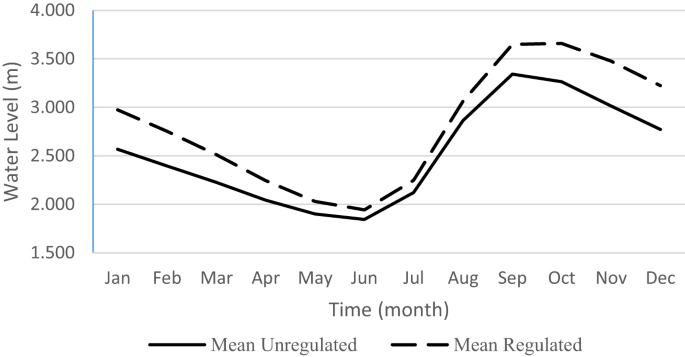
Line plot of mean water level.
Fig. 3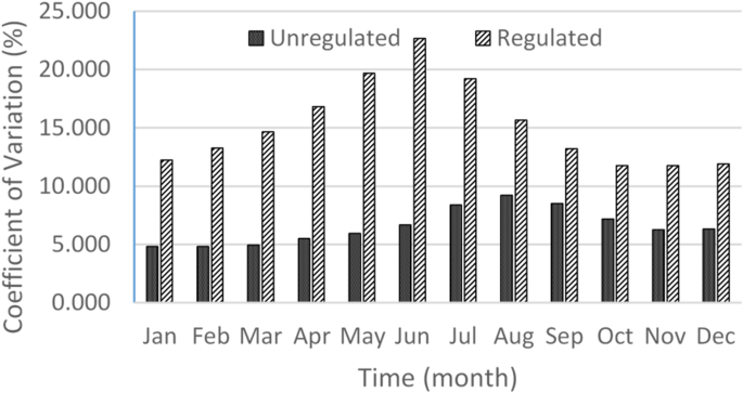
Lake water level monthly coefficient of variation.
Fig. 4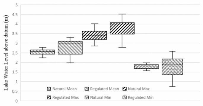
Box plots of the mean, maximum, and minimum water levels in the unregulated and regulated conditions.
During the regulated period, the lake water levels were more variable, showing more than double increment in the coefficient of variation (Fig. 3). Prior to the construction of the dam the monthly coefficient of variation of the Lake water levels were almost same for all months with some increment in the wet seasons. But after damming the monthly coefficient of variation has shown very distinct and visible differences. Even higher coefficient of variations are seen in the months of April, May, June and July. In addition to the differences observed in the magnitude of the monthly coefficient of variations between the two periods there is also a difference on the months with higher coefficient of variations. These changes have been observed because of the system change from natural to artificial. Flows in the natural system and state is governed by free outflow from the lake and the flow hydraulics through the river. But during the regulation period, it is determined artificially based on the hydropower demand and the lake state. This has increased the variability characteristics of the outflow as shown in Fig. 3. The power production demand characteristics becomes another important factor for managing the outflow. This has increased variability of the lake’s water level characteristics.
Again, clear distinctions are seen using box plots (Fig. 4) between the water levels observed during the unregulated (natural) and regulated periods. Increments in the medians, skewness, and variabilities are seen in the regulated period (Fig. 4). For example the medians of the regulated period have been seen increased as compared to their counterparts in the natural condition. The data distributions in the natural condition have been seen normal, while those for the regulated condition are skewed. Additionally, the ranges of the datasets have been increased. More compacted box plots have been seen for the unregulated period than the regulated. Larger box plots indicating wider range of variations have been seen in the regulated period than in the natural condition.
These changes have happened because of the damming and functional change made through the creation of active storage and controlled release of water from the Lake to secure water for power generation.
Again another graphical analysis using QQ plot has been used to get some more insights on the nature of the data distributions. The plots depict differences in the normality characteristics of the data sets. While the QQ plot shows a straight line for the unregulated water levels (Fig. 5), suggesting that the data distribution is normal, the same plot for the regulated water level has deviated from a straight line (Fig. 6), indicating that the data are not normally distributed. Comparison of the QQ plots, Figs. 5 and 6, provide another additional insight that the probability distribution of the lake’s water level is changed after damming.
Fig. 5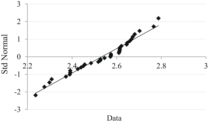
QQ Plot for the unregulated mean water level.
Fig. 6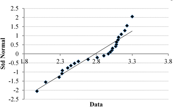
QQ plot for the regulated mean water level.
All these graphical observations are indicators of changes on the Lake’s water levels statistical characteristics. These changes could affect the Lake’s morphometry, hydrology and ecosystem characteristics. The water balance estimates and other hydrological studies should consider these changes before running to further analysis or synthesis. Hence, verifying these changes and understanding their consequences are important issues that need to be addressed.
Results of the descriptive statistics
Analyses of the descriptive statistics show that following the regulation of the Lake Outflow there are changes in the dynamics of the mean, minimum and maximum water levels of the Lake (Table 1). The regulation has increased the annual mean and annual maximum water levels of the lake by 0.25 m and 0.35 m respectively. But it has pulled down the annual minimum water level.
Table 1 Descriptive statistics of Lake Tana’s water level.
More noticeable changes are seen in the historical minimum and maximum water levels during the regulated periods. The observed historical minimum lake water levels in the unregulated and regulated periods were 1.57 m and 0.74 m respectively (Table 1). The minimum water level in the regulated period has been lower by 53% than the unregulated period. An increase of 0.5 m in the historical maximum water level of the lake was observed during the regulation period. The range, skewness, and Kurtosis of the Lake water levels were increased in the regulated conditions (Table 1). For example the lake water level range has increased from 2.45 to 3.78 m. These changes have effects on the lake’s hydrologic, morphometry and ecosystem characteristics.
The changes in the Lake water levels can significantly affect the water balance and fish productivity of the Lake. Lake Tana’s storage capacity is highly correlated with its water level indicating that a change on it brings change on the lake’s area, volume, other morphometry parameters and estimates of water balance terms. Karenge and Kolding24 have seen a remarkably high correlation between water level fluctuations, particularly the water level rises, and fish production.
Results of the inferential statistics using normality and homogeneity tests
The Shapiro–Wilk test at a 5% significance level using the Real Statistics Resource Pack version 1 is performed to check the normality of the data series. The test null hypothesis is the lake water level data series for each of the unregulated and regulated periods has normal distributions at a 5% significance level.The alternative hypothesis is the data series has not normal distributed. The analyses reveal P values of 0.32 and 0.02 for the periods of unregulated and regulated lake water levels respectively. The 0.32 P value of the unregulated period lake water level shows lack of sufficient statistical evidence to reject the null hypothesis. But the 0.02 P value for the regulated period shows the statistical evidence is sufficient to reject the null hypothesis and accept the alternative hypothesis in the regulated period. These indicate the natural, i.e., unregulated, lake water level is normally distributed, while the regulated lake water level is not normally distributed. The test confirm impacts of the outflow regulation on altering the probability distribution of the Lake Tana water level from normal to a non-normal distribution.
The Mann–Whitney method is used to test homogeneity of the data series at a 5% significance level. The test null hypothesis is that the data series is homogeneous at a 5% significance level, while the alternative hypothesis is that the data series is inhomogeneous. Using the mean lake water level data sets of the unregulated and regulated periods, a test statistic value, Uc, of 3.26 is computed using Eq. 2. For the 5% significance level, a Z score of 1.96 is read from the standard normal distribution. The computed Uc = 3.26 is higher than the Z0.975 = 1.96. This shows that the value falls in the rejection region, indicating the data sets are not homogeneous. Again, a P value of 0.003 is computed, confirming that the unregulated and regulated lake water level data sets are not homogeneous. The same results are obtained for the annual maximum and minimum lake water level series of both periods.
Discussion of the results
The lake’s mean, median and maximum water levels have increased, while the minimum water level has been decreased. During the regulated period, average increments of 0.25 m, 0.33 m, and 0.35 m have been seen for the mean, median and maximum water levels respectively. These vividly indicate that the observed changes are directly associated with the regulation of the outflow. Because in the unregulated period the water levels were normally distributed without showing either shift or trend. Neither climate change nor anthropogenic factors like land use land cover changes and water withdrawals from the Lake are claimed to be factors for the observed lake levels changes. Besides, rainfall has not shown a significant change in the past decades in the Lake Tana basin7,9,10,11 which indicates the expected impact of climate change on the lake level is minimal, if not nil.
The recent water resources developments, such as the construction of water storage dams in the Koga and Ribb Rivers and irrigation water abstractions from the lake and its tributaries, were insufficient to offset the observed mean and maximum lake water levels increment following regulation of the outflow. Many of them such as Ribb reservoir and direct pumping from Lake Tana for irrigation are very recent developments seen in the past five years. But the change has been seen before the realization of such recent developments. So, it can hardly be associated with either climate change or upstream water abstraction. The changes are the damming consequences.
The analyses mentioned above indicate that Lake Tana’s water level has acquired different statistical characteristics following the regulation of the outflow. The lake attains different water levels (Fig. 1) and different variability (Fig. 3) after the regulation of the outflow. These differences directly affect the lake’s water balance and ecosystem. It affects the lake morphometry such as depth, area, volume, and shore length which have direct effect on lake water balance and its ecosystem services. High water levels of Lake Tana enabled the expansion of the water hyacinth weed by extending its suitable habitat of shallow water to the floodplain18. However, water balance and Lake Simulation studies have not accounted for these differences12,13,14,15. Lake Tana’s water level has a very strong correlation with its area and volume8,14. A change in water level affects the lake’s surface area, volume, evaporation, direct precipitation, and other hydrological processes. In Lake Tana, a 10 cm change in its water level is equivalent to the outflow in May8. Thus homogenization of the differences should be done before estimating the water balance terms and simulating the Lake water level.
The regulation of the Lake Outflow has reduced the minimum water level by more than 50% from 1.57 to 0.74 m. The highest observed minimum water level cannot be associated with other water abstractions in the Lake and its tributaries, as it is seen in a single year and not repeated in the succeeding years when there are increased water withdrawals for irrigation purposes. If it were associated with upstream irrigation and other water withdrawals more sustained and continuously decreasing trend could have been seen. But the observation didn’t show it. Implying that the change is associated more with the control and release of water for the power generation. It has happened to maintain the required active volume storage capacity in the lake for power generation. The reduction has impacted the ship transport service for over two months in 2003. Lake Tana is navigable at the Lake water level elevation of 1784.75 m a.s.l, i.e., when the water level reading is maintained above 1.03 m from the local datum8.
Lake Tana has an extensive floodplain14. Flooding is a recurrent phenomenon in the Lake Tana basin25, primarily occurring due to the bank overflow of Inflow Rivers and the increase in the lake’s backwater flow. Controlling Lake Tana’s outflow has raised the maximum water level by 0.5 m. On one hand, this has increased the area of flooded regions in the floodplains through backwater flows and the extent of free water surface evaporation. On the other hand, it has exacerbated the spread of water hyacinth in the lake. High water levels in Lake Tana have enabled the expansion of the water hyacinth weed by extending its suitable habitat from shallow water to the floodplain18. Water hyacinth coverage was increased at a rate of 14 ha/day from August to November of 2017, and the Lake level was strongly correlated with water hyacinth spatial coverage26.
The regulation has significantly increased the range of water level from 2.45 to 3.78 m. Fluctuating lake levels can adversely affect fisheries24 indicating that assessing and evaluating the damming consequences on socio-economic and environmental aspects is necessary to ensure the sustainability of controlling and releasing water from the lake for power production. So, any hydrological analysis and synthesis on Lake Tana should consider the changes in the Lake water levels occurred due to natural and anthropogenic factors. Because heterogeneity can be introduced between data sets observed in different periods with different natural and/or artificial features. Without considering the changes and homogenising them reliable estimates cannot be obtained. Previous Lake Tana water balance and lake level simulation12,13,14,15 studies didn’t considered this fact in their analyses. Hence, updating them in view of these clearly observed changes are necessary.