Data summary
We collected 386 blood samples with matched genotype and gene expression data from the PigGTEx project [9]. The details about these blood samples were provided in Table S1. We predicted the missing sex information using MetaPred (https://github.com/FarmGTEx/metadata-prediction-v1) based on gene expression data. For the prediction of sex information, we utilized the gene expression data (transcripts per million, TPM) derived from PigGTEx project and utilized the 20-fold × 5-repeat times to obtain the prediction probability of sex information for each sample. Then, we retained the samples with the prediction probability of sex information higher than 95% for downstream analysis. For the genotype data, the low-density single nucleotide polymorphisms (SNPs) were called from the RNA-seq data using GATK (v4.0.8.1) [22]. After that, the low-density genotypes were imputed to high-density genotypes using Pig Genomics Reference Panel by Beagle (v5.1) [23]. After quality control, 2,833,585 common bi-allele SNPs (minor allele frequency (MAF) > 0.05) across samples were maintained for further analysis. The details about the processing of genotype data could be found in the PigGTEx project [9]. After quality control, 384 samples with known sex information (including 156 males and 228 females) were kept for the downstream analysis.
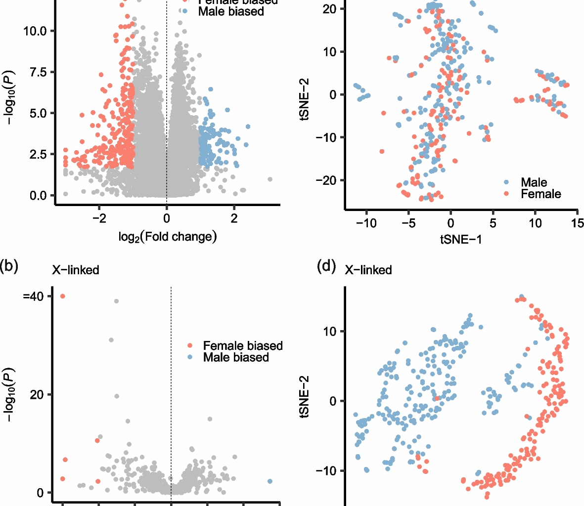
Differentially expressed genes analysis
Low expression gene (mean read counts 24]. Next, we yielded the surrogate variables (confounding factors) of normalized gene expression data except the sex using smartSVA R package (v 0.1.3) [25]. The procedure about the adjustment of confounding factors was as follow. First, we utilized the num.sv() function grouped by sex information to calculate the number of surrogate variables (including 2 surrogate variables). Next, we utilized the smartsva.cpp(n.sv = 2) function to compute the surrogate variables. After that, we adjusted the surrogate variables for normalized gene expression data using removeBatchEffect() function from limma R package (v3.60.6) [26]. We leveraged the adjusted gene expression data to perform differentially expressed genes analysis using Wilcox test method. Finally, we set the false discovery rate (FDR) 2(fold change)|> 1.5 as the threshold to obtain the sex-biased genes.
Sex-combined and sex-stratified cis-h2
To explore the similarity and difference of genetic variance of gene expression between male and female, we estimated the sex-combined and sex-stratified cis-h2 of gene expression in blood using OmiGA (v1.0.4.250515_beta2) [27]. For the processing of gene expression data, we first maintained the genes located on autosome. Next, we removed the genes with TPM 28] using edgeR R package, and then performed inversed normal transformation of the TMM. To estimate sex-combined cis-h2, we utilized the entire dataset to estimate cis-h2. To estimate sex-stratified cis-h2, we separated the genotypes and gene expression data into male and female-stratified dataset to estimate male-stratified and female-stratified cis-h2, respectively. The statistical model was as follows:
$${\varvec{y}}={\varvec{X}}{\varvec{b}}+{{\varvec{g}}}_{{\varvec{a}}{\varvec{c}}}+{\varvec{e}}$$
where \({\varvec{y}}\) is a vector of normalized expression for each gene, \({\varvec{b}}\) is covariates including the phenotype and genotype principal components (PCs) estimated by OmiGA, \({{\varvec{g}}}_{{\varvec{a}}{\varvec{c}}}\sim {\varvec{N}}\left(0,{{\varvec{G}}}_{{\varvec{a}}{\varvec{c}}}{{\varvec{\upsigma}}}_{{\varvec{a}}{\varvec{c}}}^{2}\right)\) is the cis-additive genetic effect, \({{\varvec{\upsigma}}}_{{\varvec{a}}{\varvec{c}}}^{2}\) is the cis-additive genetic variance, \({{\varvec{G}}}_{{\varvec{a}}{\varvec{c}}}\) is additive cis-genomic relationship matrix (cis-GRM) constructed by genotypes located in cis-region that around 1 Mb of the transcript start site (TSS) of gene. \({\varvec{e}}\sim {\varvec{N}}\left(0,{\varvec{I}}{{\varvec{\sigma}}}_{{\varvec{e}}}^{2}\right)\) is the residual effect, \({{\varvec{\sigma}}}_{{\varvec{e}}}^{2}\) is the residual variance. \({\varvec{X}}\) is the designed matrix for \({\varvec{b}}\).
For the phenotype and genotype PCs, we considered the PC with parameter “–dprop-pc-covar 0.001” in OmiGA. We used the parameter “–h2-model Ac” for estimating the sex-combined and sex-stratified cis-h2.
Sex-combined and sex-stratified cis-eQTL mapping
To investigate the genetic effect of gene expression in blood, we performed cis-eQTL mapping using OmiGA. For the combined cis-eQTL mapping, we utilized the whole dataset to perform cis-eQTL mapping. for the sex-stratified cis-eQTL mapping, we separated the genotypes and gene expression data into male and female-stratified dataset to conduct male-stratified and female-stratified cis-eQTL mapping, respectively. The statistical model was as follows:
$${\varvec{y}}={\varvec{X}}{\varvec{b}}+{{\varvec{s}}}_{{\varvec{g}}}{{\varvec{\beta}}}_{{\varvec{g}}}+{{\varvec{g}}}_{{\varvec{a}}}+{\varvec{e}}$$
where \({{\varvec{\beta}}}_{{\varvec{g}}}\) is the genetic effect of SNPs. \({{\varvec{s}}}_{{\varvec{g}}}\) is the vector of genotypes coding as 0, 1 and 2. \({{\varvec{g}}}_{{\varvec{a}}}\sim {\varvec{N}}\left(0,{{\varvec{G}}}_{{\varvec{a}}}{{\varvec{\upsigma}}}_{{\varvec{a}}}^{2}\right)\) is the additive genetic effect. \({{\varvec{\upsigma}}}_{{\varvec{a}}}^{2}\) is the additive genetic variance. \({{\varvec{G}}}_{{\varvec{a}}}\) is the additive GRM constructed by genotypes. The other variables are the same as statistical model of cis-h2.
Sex-interaction cis-eQTL mapping
We performed the sex-interaction cis-eQTL mapping using OmiGA. The statistical models included linear model (LM) and linear mixed model (LMM). The LMM for the sex-interaction cis-eQTL mapping was as follows:
$$\begin{aligned}{\varvec{y}}=&{\varvec{X}}{\varvec{b}}+{{\varvec{s}}}_{{\varvec{g}}}{{\varvec{\beta}}}_{{\varvec{g}}}+{{\varvec{s}}}_{{\varvec{g}}}\times {\varvec{s}}{\varvec{e}}{\varvec{x}}\boldsymbol{*}{{\varvec{\beta}}}_{{\varvec{g}}\times {\varvec{s}}{\varvec{e}}{\varvec{x}}}\\&+{\varvec{s}}{\varvec{e}}{\varvec{x}}\boldsymbol{*}{{\varvec{\beta}}}_{{\varvec{s}}{\varvec{e}}{\varvec{x}}}+{{\varvec{g}}}_{{\varvec{a}}}+{\varvec{e}}\end{aligned}$$
where \({\varvec{s}}{\varvec{e}}{\varvec{x}}\) is the vector of sex. \({{\varvec{\beta}}}_{{\varvec{g}}\times {\varvec{s}}{\varvec{e}}{\varvec{x}}}\) is the effect of sex-genotype interaction. \({{\varvec{\beta}}}_{{\varvec{s}}{\varvec{e}}{\varvec{x}}}\) is the effect of sex. The other variables are the same as statistical model of cis-eQTL mapping.
To investigate the differences and similarities between LM and LMM, we also utilized the linear model to perform sex-interaction cis-eQTL mapping. The LM was as follow:
$$\begin{aligned}{\varvec{y}}=&{\varvec{X}}{\varvec{b}}+{{\varvec{s}}}_{{\varvec{g}}}{{\varvec{\beta}}}_{{\varvec{g}}}+{{\varvec{s}}}_{{\varvec{g}}}\times {\varvec{s}}{\varvec{e}}{\varvec{x}}\boldsymbol{*}{{\varvec{\beta}}}_{{\varvec{g}}\times {\varvec{s}}{\varvec{e}}{\varvec{x}}}\\&+{\varvec{s}}{\varvec{e}}{\varvec{x}}\boldsymbol{*}{{\varvec{\beta}}}_{{\varvec{s}}{\varvec{e}}{\varvec{x}}}+{\varvec{e}}\end{aligned}$$
For the linear model, we removed the component of additive genetic effect \({{\varvec{g}}}_{{\varvec{a}}}\) in the statistical model to perform the sex-interaction cis-eQTL mapping.
We performed aggregated Cauchy association test (ACAT) [29] method to calculate the q-value (false discovery rate, FDR), and set the FDR cis-eQTL mapping, we classified genes into four categories, including male-specific genes (significant only in males), female-specific genes (significant only in females), shared genes (significant in both sexes,”Both”), and non-significant genes (not significant in either sex,”Neither”).
Phenome-wide association study (PheWAS) in pig and human
To investigate the genetic connection between sb-eQTL/eGenes and complex traits, we first performed PheWAS analysis using PigBiobank [30]. We utilized the top sb-eQTL of sb-eGenes to obtain the association of GWAS meta-analysis across 25 complex traits in pigs (Table S2). The detailed information of GWAS meta-analysis could be found in the previous study [1]. In addition, we also performed the PheWAS of sb-eGenes based on ortholog genes derived from BioMart in human complex traits using GWAS atlas [31] (https://atlas.ctglab.nl/PheWAS). We considered the Bonferroni correction (P = 0.05/number of traits) as the significant threshold.