Constructing the pangenome-derived allele databaseSearch and extraction of initial genes of interest from pangenome assemblies
Our pangenome cohort was composed of assemblies from the HPRC (92 haplotypes, excluding HG02080 due to abundant flagged regions), the CPC (114 haplotypes), the HGSVC (18 haplotypes; only PacBio HiFi assemblies were used), two telomere-to-telomere diploid assemblies (four haplotypes) and reference genomes (GRCh38 including alternative loci and T2T-CHM13). The gene coordinates used were from GENCODE version 39 based on the GRCh38 reference genome.
We constructed databases for 3,203 genes found to have copy number variation in the HPRC and CPC studies. Genes were initially organized into ‘query sets’ where each query set encompassed genes with functional or similar sequences including pseudogenes and genes with distant homology within the same gene family. The query sets were initially defined based on genes with shared name prefixes and were used to locate all similar sequences within the pangenome.
Efficient mapping methods58,59 missed alignments to sequences that contain k-mer matches and decreased genotyping accuracy when not included in our database, including small pseudogenes and diverged paralogs. To address this, we developed a sensitive and efficient scanning scheme centered on k-mer clusters to detect all similar sequences for genes of interest in the pangenome (Supplementary Notes).
The hotspots defined by k-mers often include loci mapped by multiple genes from a query set and tandemly duplicated genes. To account for this redundancy, we merged alignments that were less than 10 kb apart (together with 5 kb of flanking sequences, this merges genes within 20 kb), causing tandemly duplicated genes to be merged into a single locus. To avoid genotyping longer loci that may be split by recombination, we divided loci at the midpoints of introns exceeding 20 kb. To ensure a minimum locus length, flanking sequences were adjusted to achieve a minimum length of 15 kb. These methods aim to standardize the size of each sequence to approximate the size of LD blocks. The collection of all sequences mapped by a query set are referred to as initial matrix sequences.
Filtering and polishing initial matrix sequences and k-mers
For each genome, we first extracted k-mers found exclusively in the initial matrix sequences. We then filtered out low-complexity k-mers with a composition of at least two-thirds redundant 2-mers or 3-mers and k-mers with high (>70%) or low (60 to reduce bias in genotyping. The matrix sequences composed of a majority of filtered k-mers as well as those from HPRC nonconfident regions, truncated sequences from small scaffolds and non-telomeric sequences within 10 kb of the end of a scaffold were removed.
The initial groups of matrix sequences had sequences with low homology but similar names. Unrelated sequences from our initial groups of matrix sequences were partitioned using graph partitioning based on k-mers (Supplementary Notes).
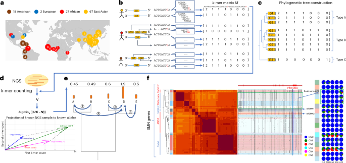
The resulting filtered sequences were labeled as PAs. There were 1,408,209 PAs for 3,351 genes in total from 3,307 partitions. This includes any additional genes not defined as duplicated in the original set that had high sequence similarity. The average PA length was 33 ± 29 kb and included protein-coding genes (69%), processed pseudogenes (20%), intronic duplications (5%) and decoys (unrelated genes that share homology and improve genotyping accuracy when included; 7%). We represented each final partition as a single matrix along with the list of low-copy k-mers specific to the matrix that passed filtration (k-mer matrix). Each row corresponds to a PA sequence. Each column corresponds to a distinct k-mer. The matrix values are the counts of corresponding k-mers in the respective PA. The counts are mostly 0 or 1 but are occasionally greater when there are low-copy repeats in the PA or the row represents a tandemly duplicated locus.
Annotation of pangenome-derived alleles
k-mer-based phylogenetic tree construction
We constructed a separate phylogenetic tree for each k-mer matrix for use in annotation and genotyping. For computational efficiency as well as consistency with our k-mer-based genotyping and annotation, we used distances based on k-mers instead of MSAs for construction.
The matrix structure (we use M to denote any arbitrary k-mer matrix) allows us to easily measure the concordance between any two sequences by their vector form, Gi and Gj, by calculating their inner product, denoted as Gi × Gj>. The norm matrix N = M × MT reflects the k-mer concordances for all sequence pairs within the matrix. We constructed a similarity matrix, S, where Si,j is the cosine similarity of Gi and Gj. Finally, we used the unweighted pair group method with arithmetic mean algorithm on S to generate the phylogenetic tree for each partition.
Clustering of pangenome-derived alleles into highly similar subgroups
For each group of sequences corresponding to a matrix, we used its corresponding phylogenetic tree for the annotation and classification of highly similar groups of alleles, which we term ‘highly similar subgroups’. The classification of highly similar subgroups is guided by two criteria: (1) a subgroup must have homology among the members. This is quantified by ensuring that the largest k-mer distance between any two members does not exceed 155 k-mers (roughly equivalent to the variation caused by five single-nucleotide variants) or a SV of approximately 95 bp; subgroups represent most common variants within ~30 kb. (2) Each subgroup must be distinct from neighboring subgroups. This is measured using a k-mer F statistic score, which must exceed 2 when compared with adjacent subgroups. In cases in which subgroups are composed of fewer than three members, the F statistic may not be reliable. We default this score to 0 for small subgroups but change the cutoff of the former criteria to 155 × 3 to detect singleton rare events.
We applied these criteria to all clades in a ‘bottom–up’ recursive approach starting from leaves to report the largest possible highly similar subgroups.
Pangenome-derived allele annotation relative to the reference genome
We annotated CNV events and duplicated alleles in the pangenome assemblies relative to the GRCh38 reference genome. This requires solving for orthology assignment61, a challenging task because PAs often align to multiple paralogs on GRCh38 and the orthologous gene identified by reference mapping may not be the most similar reference gene due to gene conversion or translocation (Figs. 1f and 2a). Here, we match PAs to their closest GRCh38 genes based on k-mer similarity. For every haplotype, we obtained pairwise similarities between the haplotype and GRCh38 PAs. We matched PAs to their most similar GRCh38 PAs, starting from the most similar pair, until all PAs were matched or failed to match (had no reference gene with >90% similarity). Matches to reference genes that had already been matched were annotated as duplications.
The PAs that formerly failed to match were likely alleles with large SVs. We attempted to map them back to GRCh38 using 100-kb flanking sequences and a two-step liftover. First, we lifted PAs to the region with the best local alignment coverage, allowing SVs in alignments. Next, we performed global pairwise alignment between PAs and the lifted region to locate the best-aligned gene considering local translocations and tandem duplications (Supplementary Notes).
Finally, to annotate the proximal duplications as well as to identify diverged paralogs that failed to match by both previous methods, we annotated PAs using gene transcripts to identify PAs containing genes, pseudogenes and putative protein-coding genes. We aligned all exons from the same matrix to PAs and, based on the exon order and alignment scores, determined the optimal combinations of transcripts for each PA (Supplementary Notes). PAs containing no exons were annotated as introns, and PAs containing only transcripts of other unrelated genes were annotated as decoys.
Classification of orthologs and paralogs in the pangenome
PAs were classified into four categories, including two types of orthologs and two types of paralogs for downstream analysis:
-
1.
Reference alleles: alleles in the same subgroup as GRCh38 alleles with almost identical sequence.
-
2.
Alternative alleles: orthologs at the same genomic locus as the reference gene but in different subgroups from GRCh38 alleles due to sequence divergence or structural variation, such as HPR, NBPF and CYP2D6.
-
3.
Duplicated paralogs (alleles): paralogs duplicated to different loci from their source genes but retaining high sequence similarity (>80% k-mer similarity), reflecting recent segmental duplications. For example, AMY1A, AMY1B and AMY1C are still often considered functionally the same despite their distinct locations.
-
4.
Diverged paralogs (alleles): paralogs duplicated to different loci from their source genes and significantly divergent (k-mers). These are characterized by highly diverse nonreference paralogs, incomplete gene duplications and new divergent processed pseudogenes. An example of diverged paralogs is at a translocation event between AMY1 and AMY2B.
Justification of the representation of pangenome-derived alleles and highly similar subgroupsComparison of pangenome-derived alleles with other genomic representations
For each PA, we compared the nearest neighbor in our pangenome database as a proxy for the optimal genotyping result of samples containing that PA to its closest GRCh38 gene based on k-mer similarity. The nearest neighbor had 94.7% fewer differences on average compared to GRCh38 matches, and 57.3% had identical nearest neighbors.
There were 38.8% of subgroups with more than three members that were identifiable by k-mers uniquely shared in the subgroup, analogous to SUNKs (Fig. 2e). For example, no SUNKs exist between SMN1, SMN2 and SMN-converted due to gene conversion (Fig. 1f).
We found that recombination or other structural variation creates unique combinations of PAs that cannot be represented during leave-one-out analysis. For example, in the amylase gene, 40% (90 of 226) of haplotypes could not be represented with the remaining subgroups, particularly those with a greater number of copies than GRCh38 (45 of 67). When all PAs devoid of SVs were considered equally in a single large subgroup, 20% (46 of 226) of haplotypes remained singleton, especially those with additional copies (26 of 67). Furthermore, new subgroups are found within different structural haplotypes, such as the PAs containing adjacent AMY1 and AMY2B due to rearrangement (Fig. 2a).
Justification of highly similar subgroups in representing population diversity
We measured the extent that highly similar subgroups capture sufficient population diversity. The average pairwise k-mer cosine similarity was 98.8% within each highly similar subgroup (one base change adds ~k differences), compared with an average 94.2% cosine similarity to the corresponding reference sequence (a 5.03× decrease). Between two phylogenetically neighboring subgroups having at least three members each, the between-group variance was 6.03× greater than the within-group variance, showing that most genetic diversity may be represented using a small number of haplotype states, as both criteria suggest that more than 80% of total population variation could be represented by highly similar subgroups.
Genotyping NGS samples with ctyperInitial solution based on linear regression
Given an NGS sample and a k-mer matrix M derived from PAs, we generate a vector V of corresponding k-mer counts from the NGS sample, normalized by sequencing coverage. We seek to find a vector X that denotes the copy numbers of all PAs and minimizes the squared distance to the k-mer counts observed in NGS data, for example, argminx (ǁMT × X − Vǁ). The integer solution through mixed-integer linear programming is NP hard6; however, the relaxed non-integer solution based on squared distances has an efficient analytic solution. Compared with absolute distance, squared distance is more suitable for the normal-like noise in NGS data62,63.
To make the solution closer to the maximum likelihood estimate, during the regression, we rescale the weights of k-mers to even out their expected uncertainty. Assuming that the observation of k-mer copy number follows a negative binomial distribution with the dispersion small enough to be distinct from Poisson63, the expected variance is roughly proportional to the square of observation; therefore, we weight k-mers by the square of the reciprocal of their observed copy number. We also apply smaller weights (adjust = 0.05) to k-mers observed in only one PA and not in NGS because they are more likely to be assembly errors.
Integer solution based on recursive phylogenetic rounding
Initial linear regression yields solutions in the form of small floating point values, in which the alleles with the highest coefficients are not necessarily those closest to query genes. However, as shown by mathematical analysis (Supplementary Notes), there are strong relationships between the initial least-error solution and the true integer solutions under a phylogenetic framework:
-
1.
Nonnegative solutions: without uncertainty in predicting k-mer copy numbers, the least-error solution should be nonnegative. Therefore, we obtain a nonnegative least-error solution via the Lawson–Hanson algorithm64.
-
2.
Total copy number estimation: the sum of the initial solutions should approximate the total number of the true integer solutions, allowing us to estimate the total gene copy number in the querying sample.
-
3.
Phylogenetic position prediction: on a binary phylogenetic tree, the branch with a shorter vector distance to the genes in the querying sample will have a larger sum of coefficients (inversely proportional to distance). This relationship enables us to predict the phylogenetic position of each gene in the query sample.
-
4.
Fractality of the least-squared error solution on a phylogenetic tree: if a solution is the least-squared error solution of the tree, it is also the least-squared error solution within each clade, allowing the greedy method to perform on the phylogenetic tree.
-
5.
Large database effect: in large databases, having more genes highly similar to query genes increases condition number and tends to distribute the total coefficients across them, resulting in smaller individual coefficients. However, the total sum of these coefficients increases, improving the precision of phylogenetic position prediction, and this effect does not plateau.
-
6.
With sequencing coverage variance for NGS at ~30-fold coverage, the model precision remains. Sequenced variance is not the primary source of error.
Given the high ‘convergence’ and fractality of the solution on the phylogenetic tree in large databases, we developed a greedy algorithm to efficiently convert non-integer solutions into integer solutions. This iterative algorithm follows a bottom–up approach, starting from the leaves and progressing toward the root. At each hierarchical level, non-integer values are rounded to the nearest integer solution that minimizes the overall residual, while any remainder is propagated to the next level. Because, at each level of the hierarchy, there are only two remainders from either branch of the tree, this solution is highly efficient. We label this approach as recursive phylogenetic rounding. The pseudocode for this algorithm (naive version and optimized version) is provided in the Supplementary Information.
Benchmarking of genotypingHardy–Weinberg equilibrium
Hardy–Weinberg equilibrium analysis was performed on autosomal chromosomes, setting the maximum copy number to two and testing for significance using the χ2 distribution.
Comparison of genotyping results to pangenome assemblies
The accuracy of PA genotypes was measured by aligning the genotyped PA sequences to the corresponding assembly (ground truth). The assembly PAs were paired with genotyped PAs by a greedy method (Supplementary Notes) and aligned using Stretcher65 for masked sequences and a pairwise alignment method distributed with Locityper41 for unmasked sequences. This determined the number of mismatched bases in unmasked regions that correspond to ctyper k-mer queries.
Classification of errors
We classified four types of errors for our benchmarking:
-
1.
False positive: the genotyping results have an additional copy;
-
2.
False negative: the genotyping results have a missing copy;
-
3.
Mistyping: copy assigned to an incorrect type;
-
4.
Out of reference: the sample has a PA that is a singleton subgroup and excluded from the genotyping database during leave-one-out analysis.
Benchmarking HLA, KIR and CYP2D genes with public nomenclatures
We labeled all IPD-IMGT and CYP2D-star annotations for PAs. HLA and KIR genes in assemblies were annotated using Immuannot66, and CYP2D6 was annotated using Pangu39. We annotated genotyped PA sequences and compared them to the assembly annotation from matched samples. The results for HLA were compared with T1K35, and the results for CYP2D6 were compared with Aldy36 (Supplementary Notes).
Population analysis of pangenome-derived allelesTotal number of duplication events from genotyping results
We calculated the total number of duplication events for each 1kGP unrelated sample from ctyper genotypes, excluding seven samples that had a population mean more than five standard deviations above the average. The total number of each reference gene including pseudogenes and pseudogene-like exonic fragments was counted in each genome and compared to that in GRCh38, excluding alternate haplotypes. Each duplication event was called if the genome had a copy number more than twice that of GRCh38, excluding decoys, introns and sex chromosome genes. The total number of duplication events was reported for each genome.
Measuring F statistic values
We used the F statistic to measure the population specificity of subgroups. The F statistic is based on the F-test, with which we obtained the variances of copy numbers within all continental populations (within-group variance) and used them to divide the variances of copy numbers across different populations (between-group variance).
Relative paralog divergence
RPD measures the mean divergences of the paralogs to other alleles, in relation to the mean divergence between only orthologs. RPD was determined for each reference gene and based on the graphic MSAs (Supplementary Notes) of PAs assigned to that reference gene as well as the ctyper genotyping results.
The divergence was first determined for each pair of PAs assigned to the same reference gene based on the alignment scores of unmasked bases (mismatch and gap open = −4 and gap extend = 0, normalized by total alignment length) from graphic MSAs. The mean divergence of orthologs was determined by averaging divergence values between the two PAs from samples with copy number = 2. Samples were divided into those with additional copy numbers (copy numbers more than the population median for a gene) and those with no additional copy numbers otherwise.
It is challenging to distinguish paralogs from orthologs in complex rearrangements (for example, Fig. 2a). To only obtain divergence values from additional copies, we performed statistical estimation based on large populations. The mean sequence divergence from samples with no additional copy numbers was used as a baseline B. When the population median copy number = Y, because there are Y(Y − 1)/2 pairs, then the total baseline is B × Y(Y − 1)/2, which is subtracted from total divergence values of samples with duplications, and Y(Y − 1)/2 is subtracted from the total number of pairs. For a sample with copy number = X, the estimated paralog divergence is (total variance − B × Y(Y − 1)/2)/(X(X − 1)/2 − Y(Y − 1)/2).
The mean paralog divergence value was determined for all samples with additional copy numbers and normalized by the mean divergence of the orthologs.
Multiallelic linkage disequilibrium
mLD is an analytic continuation of SNP-based biallelic LD to allow computing linkages between multiple genotypes on neighboring loci. We measured LD between each pair of genotypes across both loci and took the weighted average of all pairs as the product of both allele frequencies of pairs.
Expression analysis of pangenome-derived allelesDetermining transcripts for expression analysis
We first represented each gene by its major transcripts from the Matched Annotation from NCBI and EMBL-EBI67 project and then aligned individual exons. Transcripts were recursively clustered together if they overlapped with previously clustered transcripts with more than 98% overall similarity, taking the average similarity of all aligned exons from the transcripts. We considered these clusters as the same transcript even though they were from different genes. Third, for each transcript, we identified all its exons and searched for unique exons that did not overlap with exons from other transcripts. Fourth, we used these unique exons to represent each transcript and filtered out transcripts that had no unique exons (2,079 of 2,579 filtered genes were known pseudogenes). Lastly, we assigned PAs to each transcript if they contained any of the corresponding unique exons with at least 98% similarity.
Expression correction
Following precedent68, we logistically corrected the raw transcript-per-million GTEx values using the tool PEER together with the first three PCs from GTEx. For GEUVADIS samples, we obtained PCs from PLINK version 2 (ref. 69) with default settings on genotypes in chr1 (ref. 70). For cross-tissue analysis, we corrected raw transcript-per-million values using DESeq2 (ref. 71) with default settings.
Association between CNVs with gene expression
We first associated gene aggreCN with expression using Pearson correlation (linear fit). To test whether including allele-specific information improved fit, we replaced aggreCN with the ctyper paCNs to perform multivariable linear regression using paCNs as dependent variables and gene expression levels as independent variables. We compared the residuals of multivariable linear regression with residuals from the former linear fitting (F-test), reporting the one-tailed P values of the reduced residual corrected for the number of transcripts tested (n = 3,224).
Linear mixed model
We performed LMM to estimate the individual expression of each subgroup with y ≈ Xβ, where y is the total gene expression, X is copy numbers and β is subgroups, solved using ordinary least-square regression.
Alternative expression of subgroups
Paralogs were assigned to a GRCh38 reference gene based on exon annotation. We merged all other subgroups assigned to the same GRCh38 gene into a single variable separate from the subgroup then being tested. Additionally, we included paralogs assigned to other reference genes that might also influence total expression to adjust for interference. For subgroups within solvable matrices with more than ten nonzero expression values, we regressed the expression values to all variables to measure effect sizes using the R lm function72. We then compared the effect sizes between the currently tested subgroup and the other subgroups of the same gene (χ2, linearHypothesis package73), corrected for the number of total subgroups tested (n = 18,518).
Across-tissue expression comparison
We determined whether a subgroup had an alternative most-expressed tissue compared to other subgroups of the same gene, using previously gene assignment and expression filtering to calculate alternative expression of subgroups. We estimated the gene expression level of each subgroup within each of the 57 tissues in GTEx version 8 using LMM analysis. The tissue with the highest expression was compared to the tissue with the second highest expression (χ2). We then compared the results between the currently tested subgroup and all other subgroups of the same gene to see whether they had a different highest-expressed tissue. When the highest-expressed tissues were different, we tested the P value of either event by combining the P values from both sides as Pcombined = P1 + P2 − P1 × P2 and corrected for the number of tests on all tissues (n = 776,902).
Analysis-of-variance tests on gene expression
We first measured the total expression variance for each eQTL transcript in the GEUVADIS cohort, filtering out units with per-sample variance less than 0.1. Experimental noise was estimated by measuring expression variance between different trials of the same individuals (mean = 10.5% of the total variance) and excluding transcripts with experimental noise exceeding 70% of the total variance, resulting in 639 transcripts. We applied the one-in-ten rule to restrict the number of variants tested to be not greater than 45 (10% of the sample size) to avoid overfitting, filtering 18 transcripts. When there were more than 45 known eQTL variants, we used the 45 variants with the lowest P values. The valid expression variance was obtained by subtracting experimental noise from the total expression variance. Using ANOVA, we estimated the explained valid variance and adjusted the results by subtracting a baseline, defined as the mean expression variance explained by permuting the orders of all samples (estimated by the mean of 100 trials). If there were no reported eQTL variants, a value of 0 was used for known eQTL variants.
The variance explained by gene aggreCN was measured by subtracting the average of 100 ANOVA results on randomly permuted subgroups from the total explained variance by paCNs to obtain the variance explained by subgroup information.
Reporting summary
Further information on research design is available in the Nature Portfolio Reporting Summary linked to this article.