The study deploys and expands the FoodS3 model to estimate the carbon hoofprint of 3,531 US cities. Our expansion develops unique estimates of beef, chicken and pork consumption for all counties across the contiguous USA that are then allocated to census-defined ‘urban areas’. These estimates add a further link to the supply chains modelled in the FoodS3 model20. This expansion models tens of thousands of supply chains that link animal feed production, animal husbandry and animal processing to final meat consumption. This allows us to quantify the carbon hoofprints and meatsheds for each city.
Meat consumption estimates
We estimate beef, chicken and pork consumption at the county level using the National Health and Nutrition Examination Survey (NHANES)50, Center for Disease Control. NHANES is a complex, stratified bi-annual survey of the dietary habits and health of approximately 10,000 individuals. It is meticulously designed to be representative of the US population and uses weighting schemes to avoid oversampling and undersampling of demographic groups. We combine five iterations of NHANES, resulting in a sample size of 51,623 individuals. We estimate the mass of per capita beef, chicken and pork consumed using the Center for Disease Control prescribed protocols for manipulating and analysing raw NHANES data and the survey package in R Studio.
NHANES records the mass of meals consumed at home and away from home (for example, restaurants, canteens and so on). Meals are classified as standardized US Department of Agriculture (USDA) food codes. We link NHANES responses to the USDA food intake converted to retail commodity database (FICRCD)51 to disaggregate meals to individual meats. The FICRCD gives the grams of beef, chicken and pork per 100 g for each of the ~10,000 USDA food codes, which we use to estimate per capita consumption of each meat in grams per capita per day.
We develop beef, chicken and pork consumption profiles based on race/ethnicity and income level as these demographic attributes influence meat consumption. For race/ethnicity, we include Black, Latino, White and Other. Other includes all races covered in NHANES with sample sizes too limited to develop reliable consumption patterns.
For income, we use a categorical variable to estimate consumption, because of the nonlinear relationship between affluence and meat consumption52. We categorize individuals as high income if the income of their household was 200% the poverty level for a given iteration of NHANES, and low income otherwise. We choose 200% as we found statistically significant differences in meat consumption patterns above and below this threshold (Supplementary Note 2).
Combining income and race/ethnicity traits produces eight unique consumption profiles for each type of meat (for example, beef consumption by White, high-income individuals). These estimates represent national averages for each demographic group and do not necessarily capture differences in regional cuisines nor other determinants of dietary habits (for example, non-Western diets consumed by immigrants). Future work should incorporate uncertainty analysis of NHANES estimates or utilize additional data (for example, supermarket scanner data) to account for these factors (Supplementary Note 6).
Being a self-reported survey, NHANES is prone to under-reporting consumption of certain foods, including meat53. However, this issue is systematic across the survey and does not reduce its ability to capture differences in consumption patterns between demographic groups. Moreover, we adjust for under-reporting by scaling NHANES consumption to national domestic meat supplies as part of the supply–demand model (see below). Given the paucity of mass-based, city-level dietary surveys, it is not possible to compare our consumption estimates to published results. Nonetheless, NHANES is generally accepted by public health experts as a reliable estimate of US diets and its method has been replicated in other countries54. We estimate that standard errors in our consumption estimates range from 1% to 10% (Supplementary Note 2).
We combine our consumption profiles of beef, chicken and pork with demographic data from the 2017 US census to estimate aggregate demand for each meat at the county level55. We choose this year to align with the 2017 USDA Census of Agriculture, a critical data input into the current version of the FoodS3 model31. We start with demographic data at the census tract level to capture the substantial variation in income and race that often occurs within counties. Census tract estimates of household income and population by race are used to determine the ratio of average household income by race to federal poverty levels. A small number of tracts lack income data by race due to small sample sizes. For these tracts we use state-level data to calculate the poverty–income ratio. After calculating this ratio, we combine population estimates by race with appropriate consumption profiles to estimate total beef, chicken and pork consumption for 73,057 census tracts. Estimates at the tract level are then aggregated to the county.
Enhancing the food-system supply-chain sustainability (FoodS3) model
The FoodS3 model is a US-based transport model that simulates the movement of crops and livestock, connecting places of production to places of consumption20. It models the distribution of crop outputs (corn, wheat, soy, alfalfa and corn silage) from the counties of production to different nodes of downstream demand (for example, livestock and dairy production, ethanol processors, soybean crushers and flour millers), and includes the entire supply and demand of each crop. It also models the subsequent stages of demand, distributing ethanol, soymeal and flour milling byproducts to livestock producers and moving dairy milk, beef cattle, hogs and broilers to primary processors. This approach includes a data accounting component, a spatially explicit environmental impact life-cycle assessment (LCA) and a transportation optimization component. The result is a link between the downstream companies and the upstream environmental impacts of the crops/products supplied.
We expand the FoodS3 model, which previously ended at the primary processing stage of meat production20,31,56,57, to estimate the downstream supply flows of processed meat to counties where meat is consumed. We do so by first estimating the equivalent balance of total supplies and total demands of each meat type across the USA and across counties. We then deploy linear optimization that minimizes total impedance between processing facilities and final consumption locations for each type of meat produced, resulting in an estimated meatshed for each consumption county. Details for estimating the equivalent balance of total supplies and total demands are described further below.
County supply of meat
We estimate the total 2017 domestic supply of each meat type across counties based on the total annual livestock and poultry population processed at primary processing facilities (that is, broilers, finished hogs, finished beef and culled cows), state-specific typical animal mass at slaughter and the associated average dressing weights for each meat type, at approximately 61% for beef and about 75% for both pork and chicken58. We then scale the total estimated chilled-carcass weight produced in each meat-processing county to match the total US chilled-carcass weight for beef, pork and chicken58. In addition to the domestic supplies, we also include imported meat and supplies from leftover stocks from previous years (‘beginning stocks’) minus ending stocks (that is, total supplies remaining for subsequent years). Altogether, imports represent approximately 10% of beef supplied, 4% of pork and 0.3% of chicken (Supplementary Table 7).
County domestic meat demand
As mentioned above, under-reporting biases produce underestimates of actual meat consumption in NHANES than actual consumption. Additionally, NHANES-based estimates represent final consumption quantities of meat, which has several layers of loss embedded throughout the supply chain and thus is less than the total chilled-carcass weight available from processing. As a result, we use the estimated distribution across counties from the NHANES-based regression analysis (that is, proportion of each meat type consumed in each county relative to the total amount of each meat consumed in the USA) and combine with the national total chilled-carcass weight used domestically58. In doing so, we avoid the issues with NHANES systematic under-reporting biases and embedded losses, and ensure that the total amount of chilled-carcass weight demanded across counties matches the total national domestic carcass weight, with around 12 Mt, 9.5 Mt and 15.5 Mt of beef, pork and chicken carcass weight, respectively59 (Supplementary Table 7).
Total loss-adjusted meat consumption
To estimate the final total quantities of meat purchased for final consumption in each county associated with the above estimated total chilled-carcass weight demanded, we must account for the losses that occur in processing and retail. In processing, losses occur from converting chilled-carcass weights to boneless edible meat, where bones and trim are removed. Additional losses occur at retail, where a portion of the meat delivered is disposed of because of expiration or other reasons it was deemed unfit for sale, and at consumption from cooking and uneaten food waste. Supplementary Table 8 shows the losses assumed at each stage for each meat type, resulting in 1 kg of chilled-carcass weight producing 0.63, 0.59 and 0.61 kg of edible beef, pork and chicken meat purchased for final consumption, respectively, and 0.50 kg, 0.42 kg and 0.52 kg of edible beef, pork and chicken meat consumed60.
Spatial carbon hoofprint
We use the FoodS3 estimated spatially explicit emissions of meat production at primary processing facilities and track these impacts through the supply chain to downstream counties of final consumption. The spatially explicit emissions of meat production are based on the Intergovernmental Panel on Climate Change (IPCC) AR5 Global Warming Potential (GWP) characterization factors with climate carbon feedbacks, and include differentiation of practices and emission profiles of upstream crop/feed production, livestock production, processing and transport across stages, producing unique cradle-to-processing gate emission intensity (kgCO2e per kg of edible boneless meat) at each processing facility (Supplementary Figs. 8 and 9). Upstream practices in crop/feed production consider regional differences in nitrogen fertilizer application rates and types; nitrous oxide rates based on soil crop type and management practices; cover crops on irrigated and non-irrigated lands; tillage regimes for no till, reduced till and conventional intensive till and implications for fuel use; irrigation quantities, water source, irrigation system and energy source; land-use change expansion rates and emission rates, with livestock practices differentiated across manure management systems, ambient temperatures, manure excretion rates, energy use and enteric fermentation rates, and processing differentiated by electricity grid profiles31,57. These spatially explicit inventories are based on a combination of USDA, Environmental Protection Agency, US Geological Survey, national laboratory, intergovernmental and non-governmental organization data and LCA databases, with extensive methodological details published previously31,56,57,61.
Emissions are allocated to fresh meat based on economic allocation approaches, which attribute 71%, 65% and 91% to beef, pork and chicken, respectively. In addition to domestic emissions, we also include emission for imports based on the distribution of countries that each meat type is imported from62 and the respective emission intensity63.
The cradle-to-processing gate emissions (kgCO2e per kg of boneless meat) thus represent the emissions associated with producing meat, delivered to the retailer. While emissions from transport are included across feed, livestock production and processing stages, we omit transportation impacts between processing facilities and final consumption to avoid double-counting with conventional urban GHG inventories.
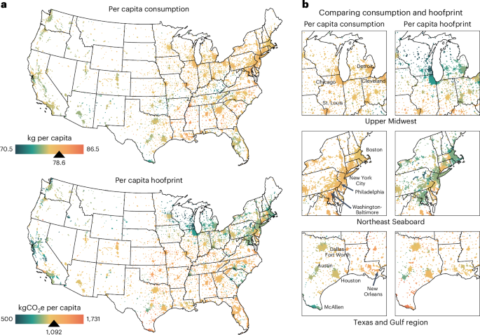
We quantify the total emissions from meat purchased and consumed in each urban area by first estimating the total emissions in each consuming county using the estimated loss-scaled quantity of each meat type sourced from each processing facility and the respective cradle-to-processing gate emission intensity. Because cities often are composed of or straddle multiple counties, we estimate the fraction of each county population within each urban area and use this to allocate a portion of the total county emissions for each meat type to each city. Summing the allocated emissions across counties in each city and dividing by the total boneless edible meat purchased results in the unique hoofprint of each city. See Supplementary Note 3 for additional details about the spatial carbon footprint methodology.
Limitations and uncertainty analysis
While spatially explicit models can explore potential impact ranges and identify geographic and stakeholder-specific hotspots and mitigation opportunities, we acknowledge several sources of uncertainty. Supply-chain estimates are inherently uncertain as a result of the opaque nature of US agriculture commodity flows. We assume that supplier–buyer relationships are solely dictated by cost and that impedance between counties (that is, difficulty or ease of shipping between counties using existing rail, road and waterways) is a reasonable proxy for this. However, supplier–buyer relationships are also influenced by contractual agreements and brand preferences.
Quantifying the standard error in the FoodS3 estimates remains challenging, as publicly available ground-truth sourcing data for validation is limited. However, consultations with stakeholders in the beef, pork and poultry industries, suggest that FoodS3 model is generally consistent with proprietary sourcing data and stakeholder expectations. Additionally, FoodS3 aligns with product-specific sourcing estimates and broader commodity-group estimates (for example, ‘animal feed’) from the Oak Ridge National Laboratory freight analysis framework (FAF5). Uncertainty is expected to be greater for locations that source small volumes from a narrow set of regions, where sourcing patterns may be more variable. Conversely, locations sourcing large volumes are more likely to draw from a broader supply region, increasing the likelihood that modelled estimates reflect average sourcing behaviour.
To test this, we use Monte Carlo scenarios to estimate variation in results from uncertainty in buyer–supplier relationships. We modelled 1,000,000 unique, mass-balanced sourcing scenarios for each of the 3,351 cities. This equates to 3,531,000,000 unique simulations across all cities. Supplementary Note 4 provides a complete description of these simulations. Monte Carlo analysis estimates a mean absolute percentage error of 26.5% for our model across all cities (Supplementary Fig. 1). This drops quickly with city size (for example, 2 and Supplementary Data 1.
We also estimate the effect of uncertainty in consumption on the results. We run 100 Monte Carlo simulations for each city (353,100 total simulations) varying consumption of each meat by each demographic group based on the statistical ranges estimated using NHANES (Supplementary Note 2). Results show that the mean absolute percentage error from baseline ranges from 0.02% to 5% for individual cities and is below 1% for all cities (Supplementary Fig. 7). Supplementary Note 5 provides a complete description of this uncertainty analysis.
Additional uncertainty from GHG inventories is also expected. Future work should overcome the computationally challenging task of quantifying this uncertainty at the county level and propagating it through downstream stages. LCA model uncertainty arises from several sources, including variability in input and output parameters (for example, material and energy types and quantities, manure management practices and environmental conditions), model selection (for example, IPCC tier 1, 2 and 3 methods; GWP characterization factors) and scenario assumptions and allocation decisions. Despite these uncertainties, our approach improves representativeness by integrating detailed, subnational production data and using tier 2 and 3 methodologies to reflect local environmental conditions. This enhances the spatial accuracy of emission estimates compared with using national averages, which may significantly overestimate or underestimate impacts. See Supplementary Note 6 for a more qualitative discussion of other sources of modelling uncertainty.
Comparisons with residential energy use and scenarioResidential energy use
We use the University of California, Berkeley’s Cool Climate Network Data (www.coolclimate.berkeley.edu) to compare the carbon footprint of residential energy use to the carbon hoofprint. The Cool Climate Network Data include estimates of emissions from in-home electricity, fuel oil and natural gas use per household for each zip code in the USA for the year 2013. The estimates were derived from multilinear regression models of fuel and electricity consumption combined with GHG intensity factors for fuels and electrical grid intensity factors from the US Department of Environment eGrid model. Details of the models underlying the Cool Climate Network Data can be found in ref. 64.
We compute total GHGs from household energy in each zip code by multiplying the number of households in each zip code by the per-household emissions. We then sum up these values for all the zip codes in each urban area and divide them by the total population to estimate the per capita GHGs from household energy in each urban area. We then compute the ratio of the per capita carbon hoofprint to per capita energy emissions for 3,531 urban areas. Spot checks with published urban GHG inventories for New York City65 and Los Angeles66 suggest that our method provides a conservative estimate of the scale of the hoofprint relative to emissions from residential energy use.
Scenarios
We explore four scenarios for hoofprint decarbonization. Scenario 1 looks at reducing edible food waste at retailers and households. We assume that baseline wastage is cut in half across both locations, leading to a decrease in total meat production as total meat demand remains constant. This means that edible beef losses are 15.1%, edible chicken losses are 13.8% and edible pork losses are 18.9%, effectively reducing emission intensity per kg of meat delivered by 18.5%, 23.4% and 16.0% respectively. Scenario 2 assumes that 50% of beef consumption is replaced by pork and chicken consumption by mass (loss-adjusted). For instance, the average annual US beef delivered to retail for final consumption would drop from 26.9 kg to 13.4 kg and average annual pork at retail would increase from 19.5 kg to 25.9 kg (chicken increases from 32.2 kg to 38.2 kg). Note that chicken required to supplant beef would decrease if substitution was based on protein and slightly increase if based on calories (pork would be largely unaffected because of similarity with beef). Scenario 3 mirrors scenario 2 except that chicken replaces pork. Lastly, scenario 4 models abstaining from meat once weekly, whereby consumption of beef, chicken and pork is multiplied by 6/7 for each city before calculating the hoofprint. As a point of comparison, we run an additional scenario considering production-side hoofprint reductions using beef silvopastures (that is, integrating trees and livestock grazing). See Supplementary Fig. 9 for results and earlier publications for methods31.
Reporting summary
Further information on research design is available in the Nature Portfolio Reporting Summary linked to this article.