Participants
A total of 24 right-handed university students (12 women, 12 men; age 21.1 ± 1.4 years) were recruited. The a-priori sample size was computed with G*Power 3.1 (Düsseldorf, Germany) for a repeated-measures ANOVA (within-factor effect size = 0.01, α = 0.05, power = 0.90, correlation among repeated measures = 0.5); the analysis indicated that a minimum of 23 participants was required. Inclusion criteria: (a) age 18–25 years; (b) regular exercisers performing ≥ 3 sessions per week, each lasting at least 30 min; (c) high interest in music or demonstrable musical understanding; (d) familiar with bicycle operation and able to cycle unaided in the laboratory; and (e) signed informed consent. Exclusion criteria: (a) history of cardiovascular, respiratory, or neurological disorders; (b) systematic cycling or competitive training within the past year; (c) participation in any music-assisted cycling intervention within the past three months; (d) acute or chronic conditions limiting exercise capacity; (e) auditory impairments or other sensorimotor deficits that could compromise data collection; and (f) current use of psychoactive medication (e.g., antidepressants, anxiolytics, or sedatives). All participants wore standardized athletic attire (short-sleeved T-shirt and shorts). After receiving a full explanation of the experimental risks, they provided written informed consent. The protocol adhered to the Declaration of Helsinki and was approved by the Beijing Normal University Ethics Committee (ICBIR_B_0213_001). Participants’ baseline characteristics are presented in Table 1.
Table 1 Characteristics of subjectsMethodsExperimental design
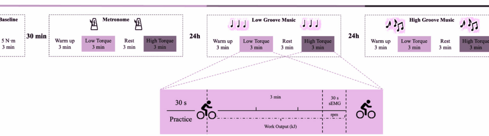
This study utilized a repeated measures design. Subjects visited the laboratory at three different time points, each visit being 24 h apart. The first visit served two purposes. The first was to establish a baseline of the subjects’ performance on music-free rides and to familiarize them with the power bike and exercise protocol. The torque was set at 5 N-m and the ride duration was 3 min, followed by a 30-min rest period. The second objective was to perform a formal riding task in the synchronized metronome condition (MT) as a Control group. At the second visit, subjects completed the riding task in the low groove music condition (LG). At the third visit, subjects completed the riding task in the high-groove music condition (HG). The experimental flow is shown in Fig. 1.
Fig. 1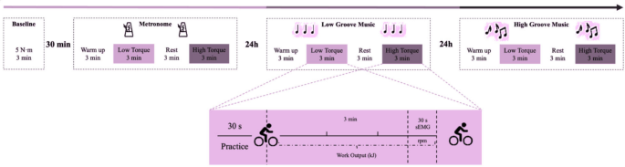
Design of the research experiment
To ensure consistency across all experimental visits (MT, LG, and HG conditions), the electromyogram (EMG) electrodes were reapplied before each session by the same trained operator, following a strict standardized protocol:
Reapply the electromyography sensor before each visit test. Skin Preparation: The skin over target muscles was shaved and cleaned with alcohol to minimize impedance variability. Electrode Placement: Sensors (Delsys wireless EMG, 10-mm inter-electrode spacing) were positioned according to SENIAM guidelines [29]. Operator Consistency: A single researcher handled all electrode placements to eliminate inter-operator variability. This approach ensured identical sensor positioning and muscle sampling across visits, guaranteeing that observed differences in muscle synergy patterns reflect true neuromuscular adaptations to rhythmic stimuli, not measurement artifacts. We confirm full adherence to best practices for EMG reliability.
Based on previous research, we selected a fixed cadence of 100 BPM to deliberately deviate from participants’ spontaneous pedaling rate (≈ 65–75 BPM), thereby imposing an external rhythmic constraint that allows us to isolate the influence of musical entrainment. In addition, 100 BPM lies within the tempo range most frequently encountered in popular music (≈ 90–110 BPM), ensuring a large and ecologically valid repertoire of tracks for future applications [29].
Deep learning-based rhythmic music screening and verification
The purpose of this study was to compare two types of music with different levels of perceived groove: high-groove music versus low-groove music. In previous studies, the assessment of groove usually relies on complex behavioral experiments, which limits the number of available music samples. To overcome this limitation, a deep learning model was trained in this study. The model was trained using acoustic features and scoring data from 264 music clips provided by Janata [30], this selection is not based on a dataset, but rather on the vocal characteristics provided by Janata. For specific details, please visit https://doi.org/10.6084/m9.figshare.30217846.v1, where we have published the full text of Janata’s article. (The Janata classification is a music research database that combines subjective perception scores with objective acoustic features. It contains 264 diverse music clips (each approximately 30 s long), which were rated on a scale of 1 to 7 by professional musicians and ordinary listeners based on the dimension of “groove.” At the same time, 21 acoustic features, such as pulse clarity and rhythmic complexity, were extracted to provide a standardized assessment benchmark for music-movement research.) and was able to assess the groove of any music clip and identify key acoustic features that affect the level of groove. Specifically, the whole process is divided into three steps. First, a Temporal Convolutional Network (TCN) model is constructed, which is used to build a dataset containing rough groove scores. Second, this dataset is utilized to pre-train a Multilayer Perceptron (MLP) model that is capable of inputting interpretable acoustic features as independent variables. Finally, the MLP model was fine-tuned on the original Janata dataset to achieve the highest accuracy. The construction strategy of the model is shown in Figs. 2 and 3. Correlation analysis of deep learning groove scoring and behavioral experiment scoring using tenfold cross-validation showed that the average R2 of the groove scoring model was 0.85, which suggests that the model’s scoring accuracy is high enough to be used for scoring instead of behavioral experiments. In addition, this study used SHAP to explore the acoustic features that contributed the most to groove movement, where the top 5 acoustic features all reflected elements of the music such as beat pattern, timbre, and chords. Detailed information is shown in Fig. 4 [31].
Fig. 2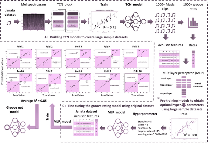
This figure shows the construction process of the music rhythm scoring model: first, a temporal convolutional network (TCN) is used to extract preliminary rhythm features from the original audio, then a multi-layer perceptron (MLP) is used to optimize these features in combination with 21 acoustic features, and finally, the model is fine-tuned on a class scoring dataset to obtain a high-precision (R2 = 0.85) rhythm scoring model
Fig. 3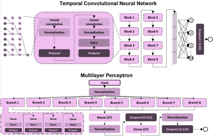
This figure shows the two-stage model architecture used for music rhythm scoring: (1) TCN (time-domain convolutional network) processes the original audio through multiple layers of dilated convolutions to capture rhythm timing features; (2) MLP (multi-layer perceptron) integrates 21 acoustic features with TCN outputs to generate the final rhythm score
Fig. 4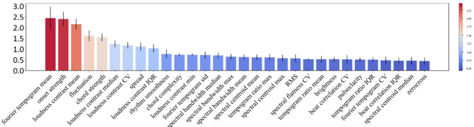
Importance ranking of acoustic features based on SHAP values
Musical segments from the top 100 English songs on the major music charts in December 2024 were rated using the model. Based on the ratings, the range of ratings for high-groove music was between 90 and 110 (top 25%), and the range of ratings for low-groove music was between 30 and 50 (bottom 25%). In this study, 11 high-groove and 11 low-groove songs were randomly selected from the 1280 scored songs. Ten college students were then recruited to subjectively assess the groove of these songs on a scale of 7. Of these songs, three high-groove songs had mean subjective groove ratings below 4.5, and two low-groove songs had mean subjective groove ratings above 4.5 and were therefore excluded from the study (Table 2). Ultimately, eight high-groove and nine low-groove songs were selected for this study. There were significant differences in the main acoustic characteristics of the songs with different groove levels (Fig. 5).
Table 2 Model scores and subjective scores of grooves of experimental entry songsFig. 5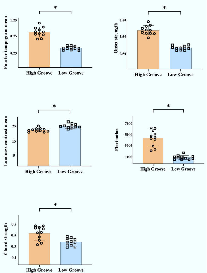
Comparison of acoustic features between music with different groove levels. Note: The acoustic feature comparison between high- and low-groove music was conducted using independent samples t-tests (for normally distributed data) or Mann–Whitney U tests (for non-normal distributions), with significance set at p
The beat frequency (BPM) of all songs was uniformly normalized to 100 BPM using Abelton Live 11 software (Abelton AG, Berlin, Germany). The music was played to the subjects through wireless Apple headphones (AirPods Pro, Apple Inc, California, USA) at a comfortable volume. The cycling task was initiated when the music started playing and completed by the end of the music. The order in which the songs were played was randomized to minimize sequential effects. In addition, for the beat Control group, this study used the GarageBand application to create an auditory beat tone of 100 beats/minute.
Recognizing grooves using deep learning models enhances the scientific validity and reproducibility of the recognition process. First, the model recognizes as much music as possible that is familiar to the current subject, which can reduce potential bias due to unfamiliarity with previous songs. Second, the model can provide important information about the effect of acoustic features on groove scores, thus improving understanding of groove [31].
Traditional methods for quantifying musical rhythm characteristics typically rely on manually extracted acoustic features (such as beat clarity and rhythm flux) or subjective behavioral scores. These methods have obvious limitations: first, manual feature extraction struggles to fully capture the multidimensional complexity of musical rhythm perception, especially higher-order nonlinear features (such as the interactive effects of syncopation patterns and dynamic compression); Second, behavioral experiments suffer from high inter-subject variability and are time-consuming, limiting the scale of music sample libraries. This study employs a deep learning model based on temporal convolutional networks (TCN) to automatically extract rhythm features most closely related to movement-synchronized behavior from raw audio signals through end-to-end learning. Its advantages include: (1) Transfer learning using 21-dimensional acoustic features analyzed within the Music Information Retrieval (MIR) framework and human rating data (R2 = 0.85), which retains the physiological significance of acoustic features (e.g., low-frequency harmonic resonance) while overcoming the sensitivity of traditional linear regression models to feature collinearity; (2) Through SHAP value analysis of the interpretability module, the acoustic features with the highest contribution to rhythm perception (such as pulse clarity and spectral flux) are identified, providing a mechanistic explanation for subsequent motion-acoustic feature coupling modeling; (3) Standardized scoring was achieved for a large sample of contemporary popular music (N = 1280), avoiding ecological validity issues caused by previous studies using limited MIDI stimuli or outdated music libraries. This quantitative paradigm provides a methodological foundation for establishing reproducible standards for music-movement coupling research in the field of movement science. For more details on deep learning and music, please refer to Appendix 1.
In addition, it should be noted that: “Rhythm” (operationalized here as BPM) refers solely to the temporal regularity and tempo of the acoustic signal, whereas “groove” is a higher-order, multi-dimensional percept that encompasses not only rhythm, but also syncopation, micro-timing deviations, dynamic accents, and timbral complexity. In other words, BPM is a necessary but not sufficient component of groove; the same BPM can yield high or low groove ratings depending on how these additional musical features are arranged. Consequently, the two constructs are measured on different conceptual levels—BPM on a one-dimensional tempo scale, groove on a composite perceptual scale that integrates rhythmic and supra-rhythmic elements [31].
Riding programs
The cycling task required subjects to synchronize as closely as possible to the groove of the music. RPM refers to the number of complete pedaling rotations completed per minute. The smaller the absolute difference between the RPM of the ride and the BPM of the music, the better the synchronization. 100 RPM was used as a target pedaling frequency to help trigger a synchronization effect in the subjects’ perception of the music groove.
In this study, a Lode Power bicycle (Lode BV, Groningen, Netherlands) was used for the cycling tasks (Fig. 6). Prior to the start of each task, subjects adjusted the seat height to a standardized level (88.3% of the inner leg length). The standardized riding protocol started with a 3-min warm-up with a torque of 2.5 N-m and a pedaling frequency of 55–65 RPM. After the warm-up, a 30-s practice phase was performed. During this period, subjects adjusted the pedaling frequency to 100 RPM based on the pedaling frequency displayed on the power bike and auditory stimuli synchronized to a musical beat. After 30 s, the pedaling frequency display was hidden and subjects completed the cycling task using only the musical groove cues. Next, subjects performed a 3-min low-torque, medium-torque, and high-torque cycling task in sequence, with a 3-min rest period after each 3-min cycling task. To determine the loading conditions where music had the greatest impact on riding performance, the power bike was set up with a fixed torque setting, with different torque levels regulating power and energy output via RPM. Low torque was set at 7 N-m for males and 4.9 N-m for females; medium torque was set at 11 N-m for males and 7.7 N-m for females; and high torque was set at 15 N-m for males and 10.5 N-m for females. The torque settings were based on the difference between male and female lower limb strength, with females being approximately 70% of the males. During the cycling phase, subjects were required to maintain a pedaling frequency of 100 RPM, synchronized to the groove of the music.
Fig. 6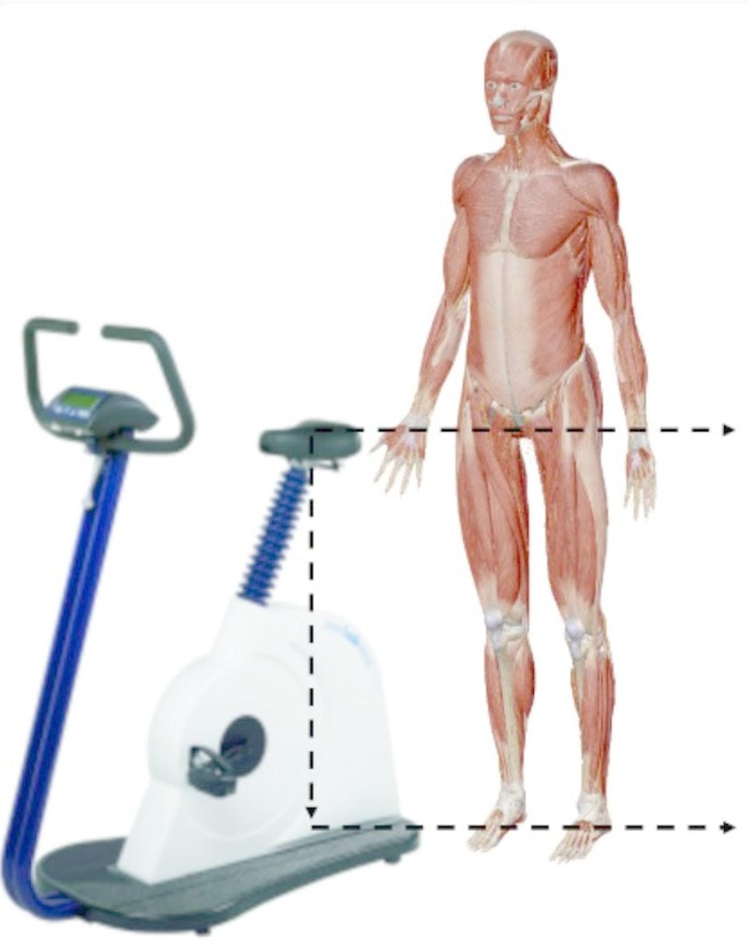
Power bicycles used in the cycling program
We presented the high-groove and low-groove conditions in a fixed sequence purely for logistical convenience; because each participant heard completely different songs in the two conditions, no track was ever repeated. Consequently, learning or habituation effects could not arise, and counter-balancing was therefore deemed unnecessary.
Measurement and calculation of joint coordination
In this study, a Qualisys motion capture system (Qualisys AB, Gothenburg, Sweden) was used to record the trajectories of the joints and cranks during the last 30 s of a 3-min cycling task under different conditions. The system consists of eight infrared cameras with a sampling frequency of 200 Hz. The experimental site was laid out as shown in Fig. 7, with the origin of the experimental environment in front of the right side of the power bike, the X-axis along the long axis of the power bike, pointing in front of the power bike from the origin, the Y-axis along the short axis of the power bike, pointing to the right side of the power bike from the origin, and the Z-axis perpendicular to the plane of the power bike, pointing to the right side of the power bike from the origin. Z-axis is perpendicular to the plane of the power bike and points to the top from the origin. Twenty-five 14-mm-diameter reflective marker points were affixed to track key areas of the head, torso, and bilateral thighs and calves using a biomechanical model of the bilateral lower extremities in Anybody software (Denmark, Copenhagen). The exact locations and abbreviated names of the marker points are detailed in Fig. 8. In addition, one reflective marker point was mounted on the outside of the right crank-pedal joint to track the crank trajectory and delineate the riding cycle (Fig. 9). The reflective marker point was secured by means of a muscle patch or a self-adhesive bandage, with bandage wrapping limited to 3 turns to avoid excessive compression of muscles and other soft tissues, which could affect athletic performance.
Fig. 7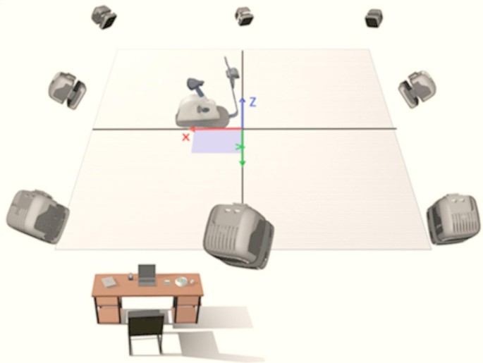 Fig. 8
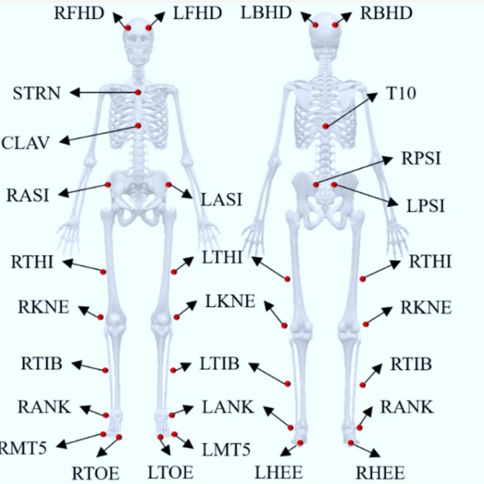
Subject reflective marker points locations based on Anybody 7.4 lower extremity model specification
Fig. 9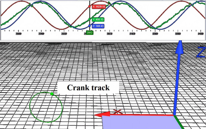
This figure illustrates the crank motion trajectory tracking method used in the experiment to determine the cycling cycle. By installing reflective markers (indicated by red arrows) on the outer side of the right pedal and combining them with a motion capture system to record its three-dimensional motion trajectory, each cycling cycle can be accurately divided (each pair of adjacent peaks represents a complete pedal cycle). This method provides an accurate time reference for subsequent joint angle and muscle coordination analysis
The kinematic data of the 25 reflective marker points were preprocessed using Qualisys Track Manager software, including naming, verification and repair of the trajectories to ensure the completeness of the marker point trajectories. Then, anybody 7.4 software was used to perform multi-link rigid body modeling and kinematic computation on the preprocessed data [32]. The lower limb model in Plug-in-gait Simple was selected to calculate the angular time series data of the torso, pelvis, hip, knee and ankle joints. In this case, the motions of the trunk and pelvic segments were referenced relative to the global coordinate system, with the motion of the trunk represented by the T10 marker point and the pelvis as its own trajectory. Finally, peaks in the crank Z-axis trajectory data were detected using an automatic peak detection algorithm written in Python. Each peak corresponds to the highest point of the pedal, and every two neighboring peaks represent one pedal cycle. Using these time points, the continuously recorded angle data was split into individual cycle data.
The vector coding technique was used to calculate the coupling angle and coordination between the lower limb joints, trunk, and pelvic segments. The angle-angle diagram was utilized to construct the angle relationship between any two segments in the time series, and the coupling angle was calculated by the vector of two consecutive time points [33]. The coupling angle is the angle of this vector with respect to the horizontal line and ranges from 0° to 360° (Fig. 10A). Depending on the coupling angle, the coordination modes are classified into four types: in-phase coordination (22.5°–67.5° or 202.5°–247.5°), which indicates that the two segments rotate synchronously in the same direction; anti-phase coordination (112.5°–157.5° or 292.5°–337.5°), which indicates that the two segments rotate in the opposite direction; proximal phase coordination (157.5°–202.5° or 337.5°–360°), indicating that motion occurs predominantly in the proximal segment; and distal phase coordination (67.5°–112.5° or 247.5°–292.5°), indicating that motion occurs predominantly in the distal segment (Fig. 10B). This study focused on exploring joint coordination between the hip-knee, hip-ankle, and knee-ankle joints in the sagittal plane of the lower extremity, as well as between the pelvis-trunk in the vertical plane.
Fig. 10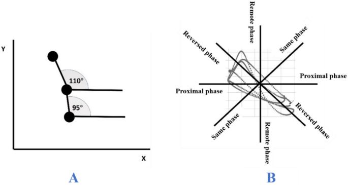
A calculation of coupling angle, B Classification of coordination modes
Vector Coding Technique (VCT) is a kinematic-based joint coordination analysis method that evaluates movement coordination patterns by quantifying the spatiotemporal relationships between adjacent joint angle changes [34]. This method converts the angular changes of two joints into vectors and calculates their phase relationships to identify specific coordination patterns, such as in-phase, anti-phase, proximal-dominant, and distal-dominant movements. Compared to traditional angle-angle plots or relative phase analysis, vector coding technique can more intuitively reveal the dynamic coupling characteristics between joints, particularly suitable for studying coordination in periodic movements such as cycling or gait [35]. In this study, the technique was applied to analyze coordination patterns between hip-ankle, knee-ankle, and pelvis-trunk joints to investigate the effects of different rhythmic music on joint coordination strategies.
Acquisition and processing of EMG data
In this study, a Delsys wireless surface EMG system (Delsys Inc., Boston, USA; electrode spacing 1 cm) was used to collect surface electromyography (EMG) data from 12 muscles of the right limb during the last 30 s of a 3-min cycling task under different conditions. The system was sampled at a frequency of 1 kHz and synchronized with a Qualisys system. The 12 muscles included: tibialis anterior (TA), medial gastrocnemius (GM), lateral gastrocnemius (GL), soleus (SOL), vastus medialis femoris (VM), vastus lateralis (VL), rectus femoris (RF), biceps femoris (BF), semitendinosus (ST), and gluteus maximus (GMX). rectus abdominis (RA), erector spinae (ES).
In the present study, only muscle synergy differences between the low groove music condition and the high torque riding in the high groove music condition were analyzed. This is partly because muscle synergy can explain the mechanisms by which musical groove affects riding performance. The metronome condition served as a control, which is inherently different from musical groove, and therefore its unsuitable for direct comparison with the musical condition. On the other hand, by comparing the effects of musical groove on riding joint coordination at different torques, low, medium and high, the study clarified that the loading condition with the greatest effect of musical groove on riding performance was high-torque riding. This provides a basis for exploring the mechanisms of musical groove on cycling performance using high-torque cycling loads.
The EMG signals were preprocessed and analyzed using the muscle synergies v1.2.5 package (Santuz, 2022) in R software (version 4.2.0, R Foundation for Statistical Computing, Vienna, Austria). Removal of averaging, bandpass filtering (4th order Butterworth 20–400 Hz) and full-wave rectification were first performed to remove low-frequency motion artifacts. Smoothing was performed by low-pass filtering with a cutoff frequency of 20 Hz. Then the root-mean-square amplitude was calculated by moving with a time window width of 20 MS and a window overlap width of 10 MS to obtain the envelope of the EMG data. Finally, the amplitude was normalized according to the maximum value for each subject; and the envelope data were time normalized and interpolated to 200 data points [36].
Calculation of muscle synergy patterns
Muscle synergies were extracted from preprocessed EMG data by a non-negative matrix factorization (NMF) algorithm. The algorithm decomposes muscle activity (D(t)) into a linear combination of time-invariant synergy vectors (Wi) scaled by time-varying activation coefficients (Ci(t)) using a set of iterative multiplicative updating rules [37]. The EMG signals can be reconstructed by the following equation:
$$D\left(t\right)={\sum }_{i=1}^{{N}_{\text{syn}}}{C}_{i}\left(t\right){W}_{i}$$
(1)
Variability Accounted For (VAF) is commonly used to test the degree of reconstruction of the reconstructed matrix with respect to the original matrix and to determine the optimal number of muscle synergies (Nsyn). i was taken sequentially from 1 to 12, as 12 muscles were recorded simultaneously in the experiment. The value of i corresponding to an initial VAF greater than 90% was chosen as the optimal number of muscle synergies per subject per experiment, and the current W and C were used as the final synergy outputs [38]. The VAF was calculated using the following formula:
$$\begin{array}{c}VAF=1-\frac{\text{SSE}}{\text{SST}}\\ SST=\sum_{i,j}{({\mathbf{D}}_{ij}-m{\mathbf{D}}_{i})}^{2},SSE=\sum_{i,j}{({\mathbf{D}}_{ij}-{\left[\mathbf{W}\mathbf{C}\right]}_{ij})}^{2}\end{array}$$
(2)
where SST is the total sum of squares and SSE is the sum of error squares, \({\mathbf{D}}_{ij}\) is the EMG data of the ith muscle at the jth time point, \({\text{mD}}_{i}\) is the average EMG value of the ith muscle, \({\left[\mathbf{W}\mathbf{C}\right]}_{ij}\) is the reconstructed EMG signal.
To characterize muscle synergy vector differences between groups, representative synergy vectors for each group were first identified by k-means clustering. The squared Euclidean metric was used, and each clustering was repeated 1000 times to select the result with the smallest sum of point-to-center-of-mass distances [39]. The number of synergistic clusters in each group was determined by calculating the Gap statistic, which is used to measure the difference in clustering compactness relative to a reference dataset with no significant clustering.
$$\text{Gap}(k)\ge \text{Gap}(k+1)-\text{sd}(k+1)$$
(3)
where \(\text{Gap}(k)\) is the gap statistic at k clusters, \(\text{sd}(k)\) is the standard deviation of the clustering compactness in the reference dataset.
In order to compare the muscle synergistic patterns between the high-groove condition and the low-groove condition, the condition with the higher number of synergistic patterns after clustering was chosen as the reference synergistic pattern in this study. For example, if the high-groove condition formed five representative synergy patterns after clustering and the low-groove condition formed four representative synergy patterns, the clustered synergy patterns of the high-groove condition were chosen as the reference. In the low-groove condition, the synergistic patterns of the low-groove condition were classified into the corresponding reference synergistic pattern categories based on the correlation between their muscle weights and the muscle weights of the reference synergistic patterns [40]. The threshold value of the correlation coefficient was 0.6, and when the correlation coefficient was greater than 0.6, the synergistic pattern could be considered to belong to the corresponding reference synergistic pattern.
In this study, the optimal number of muscle synergies, reference synergy patterns, muscle weights, and muscle activation durations were analyzed. According to the research convention, only the activation durations in the part of the activation curve where (Ci(t)) is greater than 0.3 are counted.
For more details, please refer to Appendix 2.
Statistical analysis
Data were analyzed using SPSS 26.0 software (SPSS Inc., Chicago, IL, USA). Outliers were screened using box-and-line plots, and normality was tested by the Shapiro–Wilk test [41].
Data that conformed to normal distribution were subjected to descriptive statistics using mean ± standard deviation, and one-way repeated measures analysis of variance (ANOVA) was used to compare the differences in joint coordination data among the three conditions of MT, LG, and HG. The Greenhouse–Geisser method was used to adjust the F-value when the sphericity assumption was not valid. The Bonferroni method was used for two-by-two comparisons. Effect sizes were evaluated using η2p. Paired-samples t-tests were used to compare differences in EMG data between LG and HG conditions. Effect sizes were evaluated using d. Data that did not fit the normal distribution were analyzed using the median (interquartile range) for descriptive statistics, and the Friedman test was used to compare the differences in joint coordination data between the MT, LG, and HG conditions. Two-by-two comparisons were made using the all-pairs method. The Wilcoxon signed rank test was used to compare differences in EMG data between the LG and HG conditions.
In addition, in the analysis of joint coordination data, the three riding tasks were analyzed independently because the low-torque, medium-torque, and high-torque riding tasks were relatively independent and in a fixed order. p