Figure 1 is a Hubble diagram. The points in blue show the 31 isolated galaxies used to constrain the velocity field. These are plotted in a Local Group reference frame, which we centre at a distance of 495 kpc along the line connecting the MW and M31—approximately 2/3 of the way from the MW to M31—assuming that the MW is falling towards this point with ~2/3 of the relative radial velocity of the two galaxies (as inferred in previous work8,9).
Fig. 1: Hubble diagram for the isolated galaxy sample used to trace the velocity field beyond the Local Group.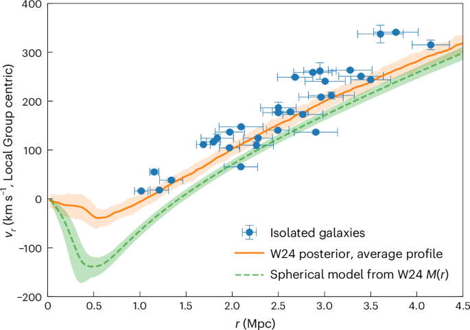
Error bars indicate 1σ measurement uncertainties on the observed distances and velocities. These velocities, together with the masses, relative positions and motions of the M31 and MW haloes, were used to constrain the initial conditions of a representative ensemble of 169 simulations of the Local Group (ref. 9; labelled W24 in the legend) within the ΛCDM paradigm. The orange line shows the mean velocity–distance relation for this ensemble. The green line shows the relation obtained from a spherical infall model based on the mean mass profile M(r) of this same ensemble. Shaded regions represent the 16th to 84th percentiles of the simulation-to-simulation scatter (the posterior scatter). Clearly, the two curves are not consistent.
The mass-weighted radial velocity profile of our ensemble of Local Group analogues,
$$\bar{{v}_{r}}(r)=\frac{1}{{M}_{{\rm{s}}{\rm{h}}{\rm{e}}{\rm{l}}{\rm{l}}}}\mathop{\sum }\limits_{\mathrm{particle}\,i\,\mathrm{in}\,\mathrm{shell}}{m}_{i}\frac{{{\bf{v}}}_{i}\cdot ({{\bf{r}}}_{i}-{{\bf{r}}}_{{\rm{L}}{\rm{G}}})}{\parallel {{\bf{r}}}_{i}-{{\bf{r}}}_{{\rm{L}}{\rm{G}}}\parallel },$$
(1)
where the sum runs over radial shells of width 50 kpc about the Local Group barycentre rLG with Mshell the total mass in each shell, and mi, ri and vi the particle masses, positions and velocities, is shown by the orange line in Fig. 1. The velocity–radius relation implied by a spherical infall model (Methods) is shown in green. Although the observational data match the actual mass-weighted velocity profile of the simulations reasonably well, the spherical model fails badly; the predicted velocities lie significantly below the data at all radii. The posterior uncertainty in the enclosed mass is insufficient to explain this; the spherical model is 5.4σ below the ensemble mean flow at 1 Mpc and 3.5σ below it at 2 Mpc. As discussed earlier, matching the observations with a spherical model implies very little mass within 4 Mpc beyond that in the haloes of two main galaxies. The sum of the two halo masses alone is at least 2 × 10¹² M⊙, and in our inference, we find ∑M200,c = 3.3 ± 0.6 × 10¹² M⊙, yet a spherical model with a total mass of just ~3 × 10¹² M⊙ within 1 Mpc and no external mass at all fits the tracer data well out to 4 Mpc (ref. 9). This is unrealistic in reasonable models of structure formation; in our ensemble of Local Group analogues, the mean mass within 4 Mpc is 4.2 × ∑M200,c. The green curve illustrates the consequence of this conflict: including this external mass in a spherical model invalidates the fit to the data.
The reason that our simulations fit the velocity field whereas a spherical model does not is that we infer a mass distribution that is not spherically symmetric but, rather, is sheet-like. In a spherically symmetric system, the net force at each radius is determined solely by the enclosed mass. This is not the case in a strongly flattened system, however. Mass located at larger cylindrical radii but near the plane exerts an outwards gravitational pull that partially offsets the inwards force experienced by the tracers, hence reducing their present-day infall velocities or, equivalently, increasing their recession velocities.
This sheet-like configuration is especially clear from our inferred posterior mean density field (the average over the ensemble of all constrained simulations). In Fig. 2, several projections of this posterior mean are shown in simulation coordinates. The top left panel shows a cylindrical view averaged azimuthally around the z axis. Clearly, there is a strong concentration of mass towards the equatorial plane of this coordinate system. We also show central slices of depth 8 Mpc of three Cartesian projections: the bottom left panel shows a view projected along the z axis, and the right two panels show the two orthogonal projections. One can see that the mass around the MW and M31 is, on average, concentrated in a sheet that is aligned with the x–y plane. Interestingly, in this coordinate system, z is misaligned by only 12 deg from the north pole of the Local Sheet of galaxies, which is itself closely aligned with the Supergalactic Plane13,14. We have inferred this mass sheet by requiring consistency between Local Group dynamics and the surrounding Hubble flow, yet it closely reflects the structure traced by luminous galaxies in the nearby Universe.
Fig. 2: Various projections of the posterior mean density ρ of the constrained simulation ensemble, normalized by the cosmic mean density \(\bar{{\boldsymbol{\rho }}}\).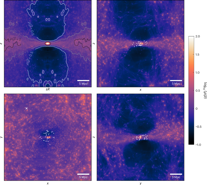
The coordinate system is centred on the MW, such that x is along the MW–M31 axis, y is towards increasing declination and z is towards increasing right ascension at the position of M31. Upper left: the density in cylindrical coordinates azimuthally averaged around the z axis with a few representative contours (these were drawn after smoothing with a 40-kpc Gaussian filter). Lower left: a projection along the z axis of a slice of depth 8 Mpc (\(| z| < 4\) Mpc). The right panels show the remaining two orthogonal projections, each corresponding to a central slice of depth 8 Mpc. White dots indicate the locations of the isolated galaxies used as flow tracers. The white cross indicates the location of the Virgo cluster. No clear overdensity is seen in this direction, and we explicitly checked for any signal with respect to azimuthal angle ϕ − ϕVirgo, finding nothing. This is consistent with the fact that the mean infall to Virgo is removed in the velocity frame of our simulations and that tidal effects due to Virgo should be relatively small over the <4-Mpc region where we have included constraints. The density visualizations use a Lagrangian sheet interpolation scheme (Methods).
The overdensity profile of the sheet is illustrated more quantitatively in Fig. 3. We find over the entire simulation region that the azimuthally averaged density on the midplane of the sheet is about twice the cosmological mean \(\overline{\rho }\), with the core of the sheet (defined as a cylindrical shell with 1 < R < 4 Mpc and ∣z∣ < 0.5 Mpc) having vertically averaged density \(\rho /\overline{\rho }=2.0{3}_{-0.78}^{+0.76}\). (Here and below quantities given in this form refer to the mean and the 16% and 84% points of the distribution over the individual simulations of our ensemble.) The thickness of the central overdensity spike, defined as the full vertical width over which the smoothed density (averaged within R < 4 Mpc and smoothed in z by a 40-kpc kernel) remains above the cosmic mean, is \(1.6{4}_{-0.45}^{+0.42}\)Mpc. Furthermore, the vertical scale height of this overdensity increases with R, so that the projected surface density of the plane increases with distance from the Local Group, as is clearly visible in the lower left panel of Fig. 2. In addition, there are strong underdensities above and below the plane, with \(\rho /\overline{\rho }=0.2{6}_{-0.14}^{+0.12}\) (for R < 4 Mpc and −8 < z < − 4 Mpc) in the direction of the Local Void15 and \(0.3{1}_{-0.11}^{+0.16}\) (for R < 4 Mpc and 4 < z < 8 Mpc) towards the local mini-void7.
Fig. 3: Azimuthally averaged density as a function of height z within thick cylindrical shells centred at the MW–M31 barycentre.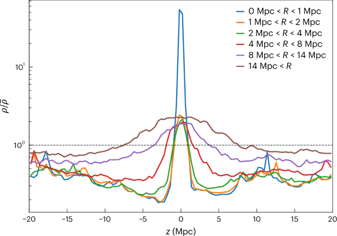
Here \(R=\sqrt{{x}^{2}+{y}^{2}}\), and the z axis is the simulation axis most nearly perpendicular to the Local Sheet.
Although we see this sheet unambiguously in the posterior mean field, it is also present in the individual realizations of the ensemble. If for each simulation we compute the eigenvalues and principal axis directions of the inertia tensor for particles with distances 2 Mpc < r < 4 Mpc (or, alternatively, 4 Mpc < r < 8 Mpc), we find the angle between the shortest axis and the z direction to be \(1{4}_{-6}^{+8}\) deg (\(1{6}_{-8}^{+10}\) deg); the average direction (the direction of the average of the minor-axis unit vectors) is just 5 deg (6 deg) from the z axis. For comparison, the angle between the shortest axis and the observed Local Sheet north pole is \(1{8}_{-7}^{+8}\) deg (\(2{0}_{-9}^{+10}\) deg), with the average direction being 13 deg (15 deg) from the pole.
Individual realizations are also strongly flattened with minor-to-major axis ratios \(c/a=0.2{4}_{-0.09}^{+0.08}\) (\(0.3{0}_{-0.10}^{+0.11}\)), intermediate-to-major axis ratios \(b/a=0.6{8}_{-0.16}^{+0.16}\) (\(0.7{2}_{-0.15}^{+0.14}\)) and minor-to-intermediate axis ratios \(c/b=0.3{6}_{-0.09}^{+0.09}\) (\(0.4{1}_{-0.12}^{+0.12}\)), measured from the mass-weighted inertia tensor in the 2 < r < 4 Mpc (4 < r < 8 Mpc) shell. c/b is substantially smaller than b/a, showing that the mass distribution around the Local Group is consistently inferred to be sheet-like rather than filamentary. An approximately spherical geometry around the Local Group is decisively rejected; across our 169 posterior samples, the maximum value of c/a is just 0.45 in the 2–4 Mpc shell, whereas a spherical distribution would have c/a ≈ 1. The configuration we have found bears a striking resemblance to the structure observed in the spatial distribution of nearby galaxies, specifically the Local Sheet13,16,17, the ‘Council of Giants’14 and the local voids above and below the sheet (the Local Void13,15,18 and a smaller local mini-void7). Our measured c/a and b/a ratios are like those found19 for galaxy positions within 8 Mpc, which yield c/a = 0.16 and b/a = 0.79. Our analysis is, thus, a dynamical demonstration that in our local neighbourhood, light approximately traces mass also on these scales.
Figure 4 shows the average peculiar velocity field. Particle momenta and masses from each realization are binned in cylindrical coordinates with ΔR = Δz = 0.5 Mpc. The stacked momentum and mass fields are then divided to obtain the mean velocity in each bin. The arrows in Fig. 4 show the resulting field. This ensemble mean flow is predominantly towards the sheet from above and below. Within the sheet, infall towards the Local Group is evident only within a radius \(R=2.5{6}_{-0.31}^{+0.33}\) Mpc (where the 500-kpc-smoothed, azimuthally averaged vR changes sign) and infall velocities are relatively low; at larger distances, peculiar velocities in the sheet are actually directed away from the Local Group. Inflow velocities are much larger towards the poles and approach or exceed 100 km s−1, even out to 8 Mpc. This strong anisotropy is not visible in our set of flow tracers because they all lie at low latitude in supergalactic coordinates, as shown explicitly in Fig. 2.
Fig. 4: The peculiar velocity field in cylindrical coordinates.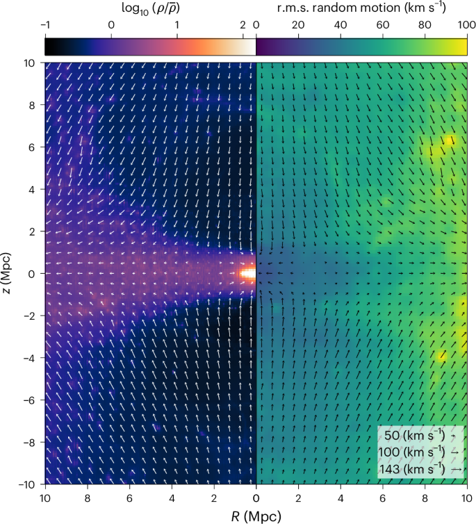
Each arrow shows the mean velocity in a ΔR = Δz = 0.5 Mpc bin. The background colouring in the left half shows the posterior mean density field (as in Fig. 2), and that in the right shows the r.m.s. scatter of the individual 500-kpc smoothed posterior velocity fields about their azimuthally averaged ensemble mean.
The background colour scale on the left side of Fig. 4 repeats the posterior mean overdensity already shown in Fig. 2. That on the right side indicates the root mean square (r.m.s.) deviation of individual 500-kpc smoothed flow fields from their stacked and azimuthally averaged ensemble mean. These random motions are small: in a cylinder with R < 5 Mpc and \(| z| < 5\) Mpc, the overall mass-weighted r.m.s. is only 33 km s−1 (in one dimension), whereas for 10-Mpc limits in both R and z, it is 58 km s−1. Within the sheet where most of our tracers lie (R < 4 Mpc and \(| z| < 1\) Mpc), it is only 22 km s−1. This shows that, although anisotropic, the overall peculiar velocity field is predicted to be very cold, even colder than the observational estimates in the papers quoted earlier. This also reflects that the posterior scatter is smallest in the region where there are the most constraints.