
SEC of molecules on MgO/Ag(001)
An STM topography of the sample is shown in Fig. 1a. We deposited Fe atoms and FePc molecules onto two monolayers of MgO atop an Ag(001) crystal. FePc molecules were shown to form an S = 1/2 system that is localized on the central Fe atom32. In addition, we include in this work a spin complex that consists of one FePc molecule that is strongly coupled to an adjacent Fe atom via one of its ligands. As shown previously33, these Fe–FePc organometallic complexes can be built using tip-assisted assembly and form a mixed-spin (1,1/2) ferrimagnet with a well-separated doublet of \({m}_{{\rm{z}}}=\pm \frac{1}{2}\), mimicking an S = 1/2 system. Both FePc and Fe–FePc constitute ideal two-level systems that allow coherent quantum control22,33. We employ both in this study, as the molecular orbital structure of FePc best demonstrates the exchange bias mechanism, while coherent control is facilitated in the Fe–FePc complex due to its resilience to inelastic electron scattering33.
Fig. 1: Molecular spins on MgO/Ag(001).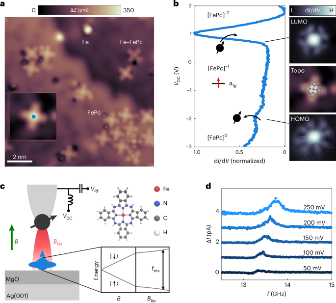
a, STM topography of the surface with the deposited Fe atoms and FePc molecules and a built Fe–FePc complex (image conditions: \(I=20\,{\rm{pA}},{V}_{{\rm{DC}}}=-100\,{\rm{mV}}\)). The inset shows a close-up topography of a single FePc molecule (2.2 nm × 2.2 nm, I = 50 pA, VDC = 100 mV). The blue dot marks the tip position of the experiments shown in b and d. b, Left: differential conductance (dI/dV) spectra acquired on the centre of the FePc (\({I}_{{\rm{set}}}=30\,{\rm{pA}},\,{V}_{{\rm{set}}}=2\,{\rm{V}},\,{V}_{\mathrm{mod}}=10\,{\rm{mV}}\)). The arrows indicate the removal (addition) of an electron leading to the transition from the [FePc]−1 (with an unpaired spin in the molecule’s a1g orbital) to the [FePc]0 and [FePc]−2 charge state. Right: the dI/dV maps show the spatial extent of both states (−2,000 mV and +400 mV) alongside the topography with an inserted chemical structure drawing. c, Left: schematic drawing of the experimental set-up with a spin-polarized STM tip above the FePc molecule atop MgO/Ag(001). A d.c. bias voltage \({V}_{{\rm{DC}}}\) and RF voltage \({V}_{{\rm{RF}}}\) are applied across the tunnel junction. The magnetic tip, realized by picking up individual Fe atoms from the surface, creates a highly localized tip field \({B}_{{\rm{tip}}}\) acting on the surface spin together with an externally applied magnetic field \(B\). Right: This is illustrated by the energy level diagram of the spin ½. Top right: chemical configuration of the FePc molecule. d, Electron spin resonance (ESR) measured on an FePc molecule for different \({V}_{{\rm{DC}}}\) showing the change in tunnel current \(\Delta I\) as a function of frequency \(f\) (ESR conditions: \({I}_{{\rm{set}}}=20\,{\rm{pA}},\,{V}_{{\rm{set}}}=60\,{\rm{mV}},{B}=484\,{\rm{mT}},\,{V}_{{\rm{RF}}}=10\,{\rm{mV}}\)). The frequency sweeps were taken at constant height (open feedback loop) and are vertically shifted for clarity.
The electronic structure of the FePc molecule is characterized in Fig. 1b by differential conductance dI/dV measurements (see also ref. 32). We observe pronounced conductance peaks around −2,000 mV (+1,000 mV) related to the process of removing (adding) an electron to the molecule34. We assign these energy positions to the highest occupied molecular orbital (HOMO) and the LUMO32,35, respectively (see also Extended Data Fig. 1 and Supplementary Section 3). Density functional theory (DFT) calculations indicate that the FePc electronic configuration involves one unpaired spin in the a1g orbital. This results from a charge transfer from the substrate ([FePc]−1) and leads to an S = 1/2 ground state22,29,32 (see also Extended Data Fig. 2 and Supplementary Section 4). The resulting magnetic spin state can be probed by ESR–STM (Fig. 1c). For ESR, the \({m}_{{\rm{z}}}=\pm \frac{1}{2}\) ground states are split by an external magnetic field B perpendicular to the sample surface
$${{hf}}_{\mathrm{res}}=g{\mu }_{{\rm{B}}}\left(B+{B}_{\mathrm{tip}}\right),$$
(1)
where \({f}_{{\rm{res}}}\) is the resonance frequency, \(h\) is Planck’s constant, \({\mu }_{{\rm{B}}}\) is the Bohr magneton and \(g\) is the g-factor. For both spin systems, \(g\) was found to be approximately \(2\) (refs. 32,33). Moreover, \({B}_{{\rm{tip}}}\) accounts for the influence of the highly localized magnetic tip field leading to a shift \(\Delta f={f}_{{\rm{res}}}-{f}_{0}\) of the surface spin’s resonance frequency. \({B}_{{\rm{tip}}}\) consists of both magnetic exchange and magnetic dipole–dipole interaction36,37, which results in different amplitude and sign of \({B}_{{\rm{tip}}}\) depending on the particular magnetic tip apex.
Motivated by SEC, which was recently observed for individual Ti atoms on MgO/Ag(001)25 in ESR–STM, we investigated the dependence of the ESR signal as a function of bias voltage \({V}_{{\rm{DC}}}\) (Fig. 1d). Here, we keep the tip–sample distance and the external field \(B\) constant while sweeping the ESR frequency. Indeed, we find a linear dependence \({f}_{{\rm{res}}}\propto {V}_{{\rm{DC}}}\) for the voltage range shown. This frequency shift can be interpreted as a contribution to the Zeeman energy by the SEC (see sketch in Fig. 1c). The intensity of the ESR signal increases with\(\,\left|{V}_{{\rm{DC}}}\right|\), mainly due to increasing tunnelling current I (Extended Data Fig. 3). For different magnetic tips, we observe that the linear voltage dependence occurs with a varying magnitude ranging from 0.5 to 8 MHz mV−1 (Supplementary Section 7). In the case of Ti atoms, a linear shift of similar magnitude was explained by a piezoelectric coupling between the magnetic tip and the surface spin25: as a consequence of \({V}_{{\rm{DC}}}\), the spin is displaced in the magnetic field of the tip, which increases or decreases \({B}_{{\rm{tip}}}\). This effect is additionally accompanied by a change in the g-factor. By contrast, in recent works by some of the authors, it was theoretically proposed that SEC can also result from transport-mediated exchange interaction29,30,31.
Nonlinear SEC
To elucidate the mechanism, Fig. 2 shows the voltage dependence of the resonance frequency for FePc molecules over a wider bias voltage range than in Fig. 1d and for different magnetic tips. For the first magnetic tip in Fig. 2a, we find that the resonance peak position starts to shift drastically and in a nonlinear manner at voltages above ≈250 mV. This shift \(\Delta f\) is accompanied by an increase in peak linewidth and amplitude as well as a change in its asymmetry. In addition, we find that \(\Delta f\) changes sign when employing a tip of opposite magnetic field direction \({B}_{{\rm{tip}}}\) (Fig. 2b). In Fig. 2c, we compare the shift of the resonance frequency \(\Delta f({V}_{{\rm{DC}}})\) for both datasets. Due to the nonlinearity, the relative shift \(\frac{\Delta f}{{f}_{0}}\) in Fig. 2c is rather large \([\pm (10-30) \%\)] compared with previous works (≈3% in ref. 25 and ≈0.2% in ref. 9). We stress that such nonlinear behaviour as found in Fig. 2 is not expected from a piezoelectric displacement model as previously used for Ti atoms25. Moreover, the latter relies on the electric-field-induced displacement of the charged surface spin, and we find this to be incompatible with the observed sign of \(\Delta f\) for FePc (Supplementary Section 6).
Fig. 2: Nonlinear SEC in the ESR spectra on FePc.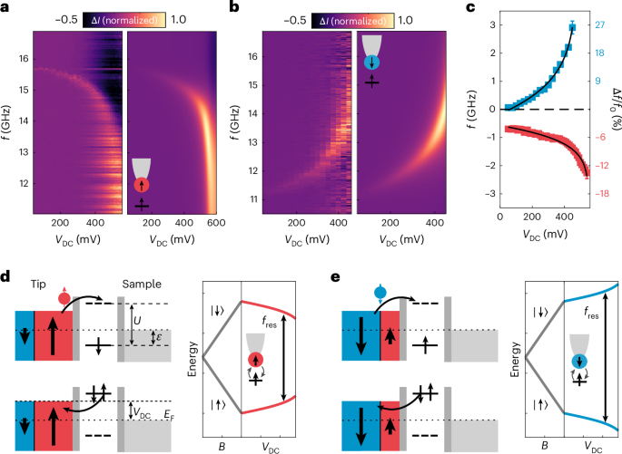
a, Colour map of the ESR signal \(\Delta I\) as a function of \({V}_{{\rm{DC}}}\) and \(f\) on a single FePc molecule. Left: experimental data (ESR conditions: \({I}_{{\rm{set}}}=10\,{\rm{pA}},\,{V}_{{\rm{set}}}=60\,{\rm{mV}},\,B=585\,{\rm{mT}},\,{V}_{{\rm{RF}}}=8\,{\rm{mV}}\)). Sharp horizontal lines are rectifications of the RF transfer function. Right: simulation according to the exchange bias model. The inset illustrates an STM tip with a spin polarization \(P > 0\) used for the simulation. b, ESR map \(\Delta I(f,\,{V}_{{\rm{DC}}})\) analogous to a, but with a different magnetic tip with \(P < 0\) (\({I}_{{\rm{set}}}=20\,{\rm{pA}},\,{V}_{{\rm{set}}}=60\,{\rm{mV}},\,B=399\,{\rm{mT}},\,{V}_{{\rm{RF}}}=8\,{\rm{mV}}\)). c, Frequency shift \(\Delta f={f}_{{\rm{res}}}-2{\mu }_{{\rm{B}}}B/h\) over \({V}_{{\rm{DC}}}\) extracted from the spectra in a (red) and b (blue). The black lines show corresponding fits of the exchange bias model, see equations (1) and (2). The second y-axis on the right-hand side displays the relative change of the resonance frequency \(\Delta f/{f}_{0}\) with \({f}_{0}=16.38\,{\rm{GHz}}\,(11.17\,{\rm{GHz}})\) for the red (blue) dataset. d,e, Schematic drawings of the virtual tunnelling processes leading to the tip-induced exchange field: The molecular spin is described via a single-impurity Anderson model (SIAM)45,46. The molecular energy levels, described by the ionization energy \(\epsilon\) and the Coulomb repulsion energy \(U\), lie between the electrochemical potential of the left spin-polarized tip electrode and the right sample electrode, separated by the vacuum tunnelling barrier and the MgO layer, respectively. The bias voltage \({V}_{{\rm{DC}}}\) moves the potential of the magnetic tip closer to the doubly occupied level for positive voltages. The polarization of the tip determines the dominating virtual tunnelling (spin up in d, spin down in e), which favour different spin states of the molecule. This leads to different \({B}_{{\rm{tip}}}\), as depicted in the energy level diagrams.
Exchange-mediated SEC
In the following, we aim to explain the behaviour by the exchange interaction between the molecule and the magnetic tip, referred to as exchange bias26,29,30,38,39,40,41,42. Notably, the nonlinear part of \(\Delta f\) emerges when the applied \({V}_{{\rm{DC}}}\) reaches the onset of the FePc LUMO shown in Fig. 1b. This indicates that the SEC mechanism is influenced by the unoccupied electronic states. A similar effect is found in quantum dot spin systems38,39,40, for instance in carbon nanotubes contacted with ferromagnetic electrodes38. The concept of exchange bias relies on virtual tunnelling processes into the excited states and was recently described in the framework of ESR–STM26,29,30,31. Figure 2d,e shows a schematic of the exchange bias in the tunnelling junction for two magnetic tips with opposite polarizations. In both cases, increasing \({V}_{{\rm{DC}}}\) raises the electrochemical potential of the tip. Subsequently, the up (down) polarization of the spin-polarized tip enhances virtual tunnelling of spin up (down) electrons into the doubly occupied state. Due to the imbalance of the spin densities in the tip electrode, the virtual tunnelling processes cause different energy corrections for the spin up and down state, which adds to the Zeeman energy. This spin-dependent energy correction can be written as38
$${B}_{\mathrm{tip}}=-\frac{P{\gamma }_{{\rm{T}}}}{2{\rm{\pi }}}\mathrm{ln}\left(\left|\frac{\epsilon -e{V}_{\mathrm{DC}}}{\epsilon +U-e{V}_{\mathrm{DC}}}\right|\right)+{B}_{0}.$$
(2)
Here, the first term is the exchange field component along the quantization axis of the surface spin. The spin polarization \(P=\frac{{n}_{\uparrow }-{n}_{\downarrow }}{{n}_{\uparrow }+{n}_{\downarrow }}\) quantifies the imbalance of the density of spin up (\({n}_{\uparrow }\)) and down electrons (\({n}_{\downarrow }\)) and sets the direction of the observed frequency shift ascribed to the tip. The coupling between the molecule and the tip \({\gamma }_{{\rm{T}}}\) can be controlled in the experiment via the conductance setpoint \({\gamma }_{{\rm{T}}}\propto G\), which alters the width of the vacuum barrier. \(e\) is the electron charge, and \({B}_{0}\) accounts for a residual tip field, stemming for instance from magnetic dipole contributions. The logarithmic relation between \({V}_{{\rm{DC}}}\) and the energy levels of the molecule,\(\,\epsilon\) (ionization energy) and \(\epsilon +U\) (\(U\) is the Coulomb repulsion energy) results in a nonlinear, diverging behaviour close to these energy levels (see Extended Data Fig. 4 and Supplementary Section 6.3 for details). Using the model, we can describe the experimental data in Fig. 2a (Fig. 2b) with a positive (negative) tip polarization: In Fig. 2c, we first use equations (1) and (2) to fit the nonlinear divergence of \(\Delta f({V}_{{\rm{DC}}})\). Here, we use the FePc HOMO level, obtained in Fig. 1b, and fix ε = 2,000 meV. We subsequently find \(\left(\epsilon +U\right)=553\pm 6\,{\rm{meV}}\) and \(477\pm 10\,{\rm{meV}}\) for positive \((P > 0)\) and negative \((P < 0)\) tip polarizations, respectively. The observed deviation can be explained by differences in the orbital energies for the two different molecules, together with variations in the setpoint conductance. Overall, the obtained \(\epsilon +U\) is in good agreement with the conductance peak associated with the LUMO from Fig. 1b. Here, we attribute the difference to the observed maximum in dI/dV (Fig. 1b, \({E}_{{\rm{L}}}\approx \text{1,000}\,{\rm{meV}}\)) to the onset of multiple orbital states inside the dI/dV peak (Extended Data Figs. 1 and 2 and Supplementary Sections 4 and 9). We note that the transition from molecular orbitals to the single-impurity Anderson model of the exchange bias model is not trivial. However, our DFT calculations (Extended Data Fig. 2) indicate that the spin-carrying orbital is a single orbital with strong d-character, which can be well approximated by a single-impurity Anderson model. We reproduce the data in Fig. 2a,b by performing full transport simulations, which aim to capture all features of the ESR–STM spectrum. The results are presented in Fig. 2a,b alongside the experimental data and show a close agreement in amplitude and resonance frequency of the peak (Extended Data Fig. 5). The convincing match between experiment and theory in Fig. 2a–c supports that the SEC is a result of the exchange bias mechanism outlined above.
Coherent spin control of molecules
To further demonstrate that a strong SEC enables all-electrical spin control, we utilize the SEC in coherent control schemes, for which we employ Fe–FePc complexes (Fig. 1a and Fig. 3a, inset). The ESR colour map in Fig. 3a shows the shift of \({f}_{{\rm{res}}}\) as a function of \({V}_{{\rm{DC}}}\). For the complex we also find an onset of nonlinear behaviour (Extended Data Fig. 6), while performing ESR at \(\left|{V}_{{\rm{DC}}}\right| > 300\,{\rm{mV}}\) remains challenging. Nevertheless, the spin complex is generally easier to use in coherent control experiments than pristine FePc (see ref. 33 and Supplementary Section 5). The pulse scheme used for Rabi oscillation measurements is depicted in Fig. 3b (refs. 21,22). The resulting coherent oscillation of the spin state leads to a change in tunnel current \(\Delta I\) as a function of the radio-frequency (RF) pulse duration \(\tau\) (ref. 21):
$$\Delta I=A \sin \left(\varOmega \tau +\phi \right) {{\rm{e}}}^{-\tau /{T}_{2}}.$$
(3)
Fig. 3: Spin–electric Rabi detuning on an Fe–FePc complex.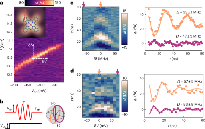
a, ESR colour map \(\Delta I\left(f,\,{V}_{{\rm{DC}}}\right)\) on the Fe site of an Fe–FePc complex (ESR conditions: \({I}_{\mathrm{set}}=6\,\mathrm{pA},\,{V}_{\mathrm{set}}=-60\,\mathrm{mV},B=469\,\mathrm{mT},\,{V}_{\mathrm{RF}}=10\,\mathrm{mV}\)). The chemical structure of the Fe–FePc is overlaid on the inset topography. The added Fe atom is highlighted by a red arrow, marking the site at which the measurements shown in c and d were performed. White arrows indicate the detuning in frequency \({\rm{\delta }}f=f-{f}_{\mathrm{res}}\) and voltage \({\rm{\delta }}V={V}_{\mathrm{DC}}-{V}_{\mathrm{set}}\) from the resonance. b, Left: schematic drawing of the Rabi pulse scheme. The RF signal consists of an RF pulse with duration \(\tau\) and amplitude \({V}_{{\rm{RF}}}\) followed by an off-time \({\tau }_{{\rm{off}}}\). The total cycle time \({\tau }_{{\rm{cycle}}}=\tau +{\tau }_{{\rm{off}}}\) is kept constant, and a d.c. voltage \({V}_{{\rm{DC}}}\) is applied continuously for readout. Right: Bloch sphere representation of the spin evolution on resonance (orange) and off resonance (purple). c, Rabi oscillations for different frequency detuning \({\rm{\delta }}f\) (Rabi conditions: \(\,{I}_{\mathrm{set}}=4\,\mathrm{pA},\,{V}_{\mathrm{set}}=-60\,\mathrm{mV},\,\)\(B=473\,\mathrm{mT},\,{V}_{\mathrm{RF}}=60\,\mathrm{mV},\,\)\(f=14.04\,\mathrm{GHz},\,{\tau }_{\mathrm{cycle}}=\,250\,\mathrm{ns}\)). Left: colour map of \(\Delta I\) as a function of \({\rm{\delta }}f\) and \(\tau\). The arrows refer to the traces shown on the right. Right: single traces on (orange) and off (purple) resonance, plotting \(\Delta I\) as a function of \(\tau\). Solid lines are fits based on equation (3) (see Extended Data Table 1 for the parameters). Traces are vertically shifted for clarity. d, Rabi oscillations for detuning the voltage \({\rm{\delta }}V\) instead of \({\rm{\delta }}f\) (Rabi conditions: \({I}_{\mathrm{set}}=5\,\mathrm{pA},\,{V}_{\mathrm{set}}=-60\,\mathrm{mV},\,\)\(B=450\,\mathrm{mT},\,{V}_{\mathrm{RF}}=20\,\mathrm{mV},\,\)\(f=14.25\,\mathrm{GHz},\,{\tau }_{\mathrm{cycle}}=\,400\,\mathrm{ns}\)). Left: colour map of \(\Delta I({\rm{\delta }}V,\tau )\). Right: single traces analogous to c.
With the amplitude \(A\), the Rabi rate \(\varOmega\), the Rabi phase \(\phi\) and phase coherence time \({T}_{2}\). Moreover, detuning from resonance \({\rm{\delta }}f=f-{f}_{\mathrm{res}}\) leads to a change in both amplitude \(A\) and Rabi rate \(\varOmega\) of the observed oscillation:
$$\begin{array}{cc}\varOmega =\sqrt{{\varOmega }_{0}^{2}+{{\rm{\delta }}f}^{2}}, & A={A}_{0}\frac{{\varOmega }_{0}^{2}}{{\varOmega }^{2}}\end{array}.$$
(4)
Here \({A}_{0}\) and \({\varOmega }_{0}\) are the parameters at \({f}_{{\rm{res}}}\). Consequently, the Rabi oscillations \(\Delta I(\tau )\) can be tuned by \({\rm{\delta }}f\), resulting in the typical chevron pattern (Fig. 3c). Utilizing the SEC, we now realize an all-electrical detuning via a change in voltage \({\rm{\delta }}V={V}_{\mathrm{DC}}-{V}_{\mathrm{set}}\) (Fig. 3d) while keeping \({\rm{\delta }}f=0\). We obtain a chevron pattern as well for \(\Delta I(\tau ,{\rm{\delta }}V)\), in which the amplitude \(A\) (Rabi rate \(\varOmega\)) decreases (increases) for increasing |\({\rm{\delta }}{V|}\). Compared with the frequency tuning, the pattern is slightly distorted. We attribute this to a linear contribution to \({\varOmega }_{0}\propto {V}_{\mathrm{DC}}\) predicted for spin resonance in the exchange bias model29,30. In addition, we expect a dependence of the amplitude with tunnelling current \(A\propto I\propto\) \({V}_{{\rm{DC}}}\) (see Supplementary Section 10 for details).
Coherent control of a molecule dimer
Finally, we realize the SEC detuning in a two-spin system. In Fig. 4a, two complexes are brought into proximity using tip-assisted manipulation to establish a coupled spin system. The resulting configuration (Fig. 4b) consists of a readout spin \({S}_{1}\) that is ferromagnetically coupled to the second spin \({S}_{2}\) mainly through Heisenberg exchange interaction \(J\) (Extended Data Fig. 7 and Supplementary Section 11). Because the coupling is substantially smaller than the Zeeman energy, the system exhibits four distinct energy levels (Fig. 4c). The two resulting ESR transitions \({f}_{{\rm{I}}}\) and \({f}_{{\rm{II}}}\) (Fig. 4c,d) primarily reflect the alignments of \({S}_{2}\) in either |↑〉 and |↓〉 state43,44. \({f}_{{\rm{I}}}\) and \({f}_{{\rm{II}}}\) shift again as a function of \({V}_{{\rm{DC}}}\), with the exchange bias from the tip acting on \({S}_{1}\). The energy splitting \({{f}_{\mathrm{II}}-f}_{{\rm{I}}}\,\approx \,130\,\mathrm{MHz}\) remains constant across the whole voltage range, indicating that the spin–spin coupling between \({S}_{1}\) and \({S}_{2}\) is unaffected by the SEC. In the corresponding Rabi oscillation measurements (Fig. 4e), we now tune from \({f}_{{\rm{I}}}\) to \({f}_{{\rm{II}}}\) by changing \({\rm{\delta }}f\), which leads to two chevron patterns. The weaker intensity of the left chevron arises from the low thermal population of the excited state \(|\downarrow {{\rangle }}\) of \({S}_{2}\). Again, the SEC enables all-electrical detuning via a change in voltage \({\rm{\delta }}V\) (Fig. 4f). The main limitation in this approach is the increased tunnelling current at higher voltages, which induces spin relaxation and decoherence21,22. However, the bias-controlled exchange field still permits to tune from the first transition (\({\rm{\delta }}V\approx 5\,\mathrm{mV}\)) to the second (\({\rm{\delta }}V\approx -80\,\mathrm{mV}\)).
Fig. 4: Spin–electric Rabi detuning in a coupled spin system.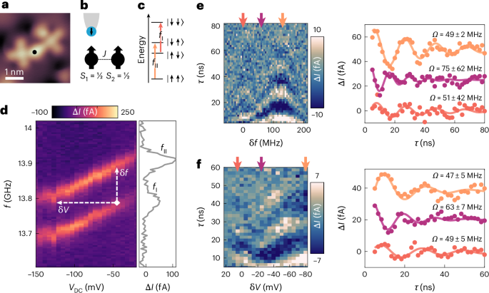
a, Topography of two coupled Fe–FePc complexes (image conditions: \(I=10\,{\rm{pA}},\,{V}_{{\rm{DC}}}=-100\,{\rm{mV}}\)). The black dot marks the tip position of the subsequent measurements. b, Schematic drawing of the two spin ½ with their exchange coupling \(J\) and the tip above the first spin \({S}_{1}\). c, Schematic energy level diagram of the combined spin states with the two ESR transitions \({f}_{{\rm{I}}}\) and \({f}_{{\rm{II}}}\). d, ESR colour map \(\Delta I(f,\,{V}_{{\rm{DC}}})\) measured on the coupled spin system (ESR conditions: \({I}_{{\rm{set}}}=8\,{\rm{pA}},\,{V}_{{\rm{set}}}=-40\,{\rm{mV}},{B}=462\,{\rm{mT}},\,{V}_{{\rm{RF}}}=10\,{\rm{mV}}\)). A single frequency sweep (right) at \(-50\,{\rm{mV}}\) reveals two distinct peaks corresponding to \({f}_{{\rm{I}}}\) and \({f}_{{\rm{II}}}\), that is, transitions corresponding to different spin states of the remote spin \({S}_{2}\). White arrows indicate the detuning in frequency \({\rm{\delta }}f\) and voltage \({\rm{\delta }}V\). e, Frequency detuning of Rabi oscillations (Rabi conditions: \({I}_{{\rm{set}}}=8\,{\rm{pA}},\,{V}_{{\rm{set}}}=-40\,{\rm{mV}},{B}=458\,{\rm{mT}},\,{V}_{{\rm{RF}}}=80\,{\rm{mV}},{f}=13.97\,{\rm{GHz}}\)). Left: colour map of \(\Delta I\) as a function of \({\rm{\delta }}f\) and \(\tau\). The pattern shows two chevrons corresponding to the two ESR transitions. The arrows at the top refer to the single traces to the right. Right: single traces of \(\Delta {I}\) versus \(\tau\) for three \({\rm{\delta }}f\). Solid lines show fits to the circular datapoints based on equation (3) (see Extended Data Table 1 for the parameters). The traces were shifted vertically for clarity. f, Electric detuning of Rabi oscillations, analogous to e (Rabi conditions: \({I}_{{\rm{set}}}=8\,{\rm{pA}},\,{V}_{{\rm{set}}}=-40\,{\rm{mV}},{B}=462\,{\rm{mT}},\,{V}_{{\rm{RF}}}=70\,{\rm{mV}},{f}=14.04\,{\rm{GHz}}\)). Left: colour map of \(\Delta I({\rm{\delta }}V,\tau )\) showing the continuous electrical tuning from one ESR transition to the other. Right: \(\Delta I\) as a function of \(\tau\) for three different \({\rm{\delta }}V\) (also see Supplementary Section 12).