
Spatiotemporal THz field mixing in scattering media
We begin addressing how fields at source and detection planes are connected by a complex combinatory matrix element of a scatterer precisely for the case of broadband pulse illumination. We define the input-output field relationship via the space-time impulse response of scattering media, \(\:{T}_{x}\left(x,y;{x}^{{\prime\:}},{y}^{{\prime\:}};t,{t}^{{\prime\:}}\right)\), as
$$\:{E}_{d}\left({x}^{{\prime\:}},{y}^{{\prime\:}},{z}_{d};{t}^{{\prime\:}}\right)=\iiint\:{T}_{x}\left(x,y;{x}^{{\prime\:}},{y}^{{\prime\:}};t,{t}^{{\prime\:}}\right){E}_{s}\left(x,y,{z}_{s};t\right)dxdydt$$
(1)
where, \(\:{E}_{d}\left({E}_{s}\right)\) is spatiotemporal field distribution at the detection/source plane in the cartesian coordinates defined by \(\:({x}^{{\prime\:}},{y}^{{\prime\:}},{z}_{d})/(x,y,{z}_{s}\)), respectively. In frequency domain \(\:\omega\:\), Eq. (1) reads as follows,
$$\:{\stackrel{\sim}{E}}_{d}\left({x}^{{\prime\:}},{y}^{{\prime\:}},{z}_{d};{\upomega\:}\right)=\iint\:{\stackrel{\sim}{T}}_{x}\left(x,y;{x}^{{\prime\:}},{y}^{{\prime\:}};{\upomega\:}\right){\stackrel{\sim}{E}}_{s}\left(x,y,{z}_{s};{\upomega\:}\right)dxdy$$
(2)
where \(\:{\stackrel{\sim}{E}}_{d}\), \(\:{\stackrel{\sim}{E}}_{s}\) denote the time-Fourier transform of the fields at detection, source plane and \(\:{\stackrel{\sim}{T}}_{x}\left(x,y;{x}^{{\prime\:}},{y}^{{\prime\:}};{\upomega\:}\right)\) represents coherent transfer function for a scattering sample.
THz source providing an ultrafast broadband pulse with a duration shorter than Thouless time (the typical time scale over which light diffuses across the medium ) results in randomised field transient in both space and time after propagating through scattering media44,45. In Fig. 1, we recorded the transmitted time-resolved THz field distribution in response to Gaussian beam illumination on the scattering sample (sample details are in supplementary S1), as shown in the schematic (Fig. 1a). As expected, scattering introduces a time-dependent morphology of the scattered field profile. Specifically, the THz field distribution resulted in complex spatial interference patterns in the transmission (Fig. 1b). The evolution of the spatial field on an ultrafast time scale shows the transition from the ballistic to the diffusive scattering regimes. Initial spatial THz field profiles at 8.85 ps and 9.45 ps show relatively more uniformity, indicating a ballistic propagation of THz waves associated with a low statistical occurrence of photon scattering, i.e., the THz field maintains its spatial momentum content. As time progresses, the diffused photons emerge, leading to an entirely randomization of the spatial field profiles due to several scattering occurrences inside the medium, shown by the spatial frames at 10.35 ps, 14.4 ps, 15 ps, and 18.9 ps. Also, the scattering process becomes more apparent in the temporal progression of distinct pixels that constitute the considerably broadened pulses in conjunction with the different time delays. However, the overall observed time delay in the pulses can be attributed to the thickness of the scattering sample (5.53 mm). As a result of the dispersive characteristics inherently present in scattering media, the temporal widening of a scattered pulse occurs concomitantly with the attenuation of its peak values. The primary cause of attenuation in the scattered pulses is attributed to the scattering of high-frequency components of the impinging pulse, as illustrated in Fig. 1c. The measured values of the mean free path (\(\:{l}_{s}\)) for the sample are shown in Fig. 1d. In our experiments, we observed the variation of \(\:{l}_{s}\left(\omega\:\right)\) ranging between 1 mm and 10 mm within the source bandwidth. Note that because the scattering media is near-field coupled with the detector, scattering can appear highly inhomogeneous in spectral properties at the output. The spatial-spectral profiles of the THz field at 0.2–0.7 THz (Fig. 1e) exhibits the formation of broadband speckles, characterised by subwavelength spot size and disordered phase distribution. We highlight that the detection is near-field coupled with the scattering media, hence, the resolution is not bounded by the wavelength. Additionally, in our experiment, the THz source spectrum extends up to ~ 1.5 THz (supplementary figures S1 and S4), but multiple scattering attenuates higher frequencies, limiting the effective spectrum to S1(c)); thus, analysis is performed in the 0.2–0.7 THz range where SNR is optimal and spatio-spectral characterisation is more reliable.
Fig. 1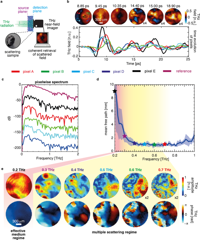
Broadband speckle formation of THz fields. (a) Schematic showing the projection of a pulsed THz field at the source plane of the scattering sample and the collection of the scattered field via a time-domain THz imager. (b) Spatiotemporal THz field transmission through scattering samples exhibits temporal distortion, as shown in the pixel-wise time evolution of the pulses and random modulation in the spatial field distributions (video 1). Field amplitude is plotted 4 times the original spatial field at \(\:14.40\:\text{p}\text{s}\), \(\:15.00\:\text{p}\text{s}\), and \(\:18.90\:\text{p}\text{s}\). (c) The pixel-wise spectrum of scattered fields corresponds to the pulses shown in a. (d) Mean free path of the scattering sample within the THz source bandwidth (e) The spatial multiplexing of broadband THz fields and phases illustrates the broadband speckle synthesis within the THz source bandwidth (video 2).
Scattering media characterisation using knife-edge wavefront shaping
The core idea is to provide a unique scattering association to different shielding portions of the broadband THz field illumination (as per ref46,47) with a knife-edge moving in the near-field of the scatterer. The scatterer waveform obtained by the 2D time-domain detection set is used as a base to reconstruct a 1D transmission matrix. Once the transmission matrix is known, the image of any 1D object can be deterministically retrieved. Figure 2a illustrates a typical setting for a knife-edge (a thin conductive blade clipping a Gaussian beam) scan, where the THz near-field imager collects scattered fields from the sample partially illuminated. We can write the spatiotemporal field profile (\(\:{E}_{s}\)) generated by the specific placement of the knife at the source plane as,
$$\:{E}_{s}\left(x,y,{z}_{s};t\right)\propto\:\text{K}\left(x{,y}_{o},{z}_{s}\right){E}_{in}\left(x,y,{z}_{s};t\right)$$
(3)
where \(\:\text{K}\left(x,{y}_{o},{z}_{s}\right)\) represents the point-wise spatial response of the knife-edge, which is defined as a one-dimensional Heaviside step function in the transverse direction with a fixed coordinate position \(\:{(y}_{o},{z}_{s})\) and \(\:{E}_{in}\) is the time-resolved Gaussian beam profile from the source. The knife-edge used in our setup is a thin conductive blade with micron-scale thickness at the sharp edge, placed approximately parallel to the scattering media input facet, and transversally translated, as shown in Fig. 2(a). Initially, we characterised the spatial beam profile for the reference THz field (included in the supplementary figure S4) to normalise the results. The key idea here is that (Fig. 2a), because of the near-field coupling, the knife-edge can selectively couple with a relatively large number of modes in the scattering volume (i.e. discernible scattering outputs) not necessarily accessible through far-field illuminations.
Fig. 2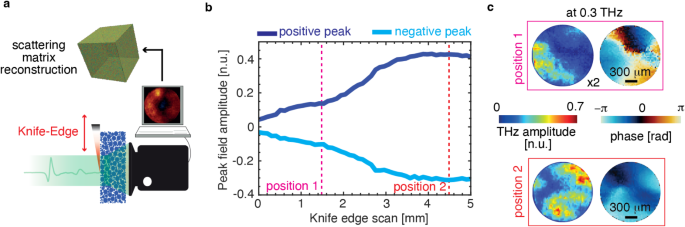
Scattering media characterisation using knife-edge wavefront shaping. (a) Schematics of the experimental setup showing a knife-edge shapes the impinging THz wavefront at the front end of the scattering medium (8% fractional mass concentration of Silicon microparticles embedded in paraffin) and corresponding scattered fields are collected using a THz time-domain imager placed within the near-field region. By combining the transmitted fields corresponding to the various knife-edge positions, the space of potential 1D spatiotemporal images could be derived and further constructed as a hyperspectral combinatory scattering matrix to characterise the scattering sample. (b) variation of pulse peak value with respect to the various transverse position of knife-edge. (c) spatial field amplitude and phase profile at 0.3 THz corresponding to knife-edge position 1 and 2 (dashed lines shown in b).
Figure 2b illustrates the variation in positive and negative peak values of the pulse as a function of the transverse position of the knife-edge. The scan axis is oriented to uncover more THz field as the translation increases. In the spectral domain, the spatial field amplitude and phase distribution at 0.3 THz, corresponding to the input wavefronts generated by two different knife-edge positions (at 1.5 mm and 4.5 mm), are shown in Fig. 2c, highlighting the influence of the scattered field from the knife-edge positions.
We can write fields at the source and detection plane as vectors \(\:{e}_{s}\in\:{\mathbb{C}}^{S\:\times\:1}\) and \(\:{e}_{d}\in\:{\mathbb{C}}^{D\:\times\:1}\), and define a scattering combinatory transfer matrix as \(\:{\varvec{T}}_{ds}\in\:{\mathbb{C}}^{S\:\times\:D}\), for each frequency ω. S and D represent the number of independent pixels (or segments) that sample the input and output field plane, respectively. For R number of independent spectral sampling points, T is a \(\:{\mathbb{C}}^{S\:\times\:D\times\:R}\) three-dimensional matrix, defined as \(\:{\varvec{T}}_{ds}\left({\omega\:}_{r}\right)\). For the given r-th spectral mode, the linear relationship between generic s-th source and d-th detection spatial segments reads as follows,
$$\:{e}_{d}\left({\omega\:}_{r}\right)=\sum\:_{s}{\varvec{T}}_{ds}\left({\omega\:}_{r}\right){e}_{s}\left({\omega\:}_{r}\right)$$
(4)
Further, for each i-th position of the knife-edge, we collect the corresponding \(\:{e}_{d}^{\left(i\right)}\left({\omega\:}_{r}\right)\) and column-wise stack in a measurement matrix \(\:\varvec{M}\left({\omega\:}_{r}\right)\in\:{\mathbb{C}}^{D\:\times\:P}\) and corresponding synthesised THz wavefront in decomposition matrix \(\:\varvec{X}\left({\omega\:}_{r}\right)\in\:{\mathbb{C}}^{S\:\times\:P}\), where P is the number of wavefronts modulated by the edge of the knife. To identify the transfer matrix at frequency \(\:\omega\:\), we set up a least square optimisation problem as,
$$\:{\varvec{T}}_{r}^{\dagger}\left({\omega\:}_{r}\right)=\text{a}\text{r}\text{g}\text{m}\text{i}{\text{n}}_{\:{T}_{r}\in\:{\complement\:}^{S\:\times\:D}}\:\frac{1}{2}\:{\left\| {\varvec{M}\left({\omega\:}_{r}\right)}^{\dagger}-{\varvec{X}\left({\omega\:}_{r}\right)}^{\dagger}{\varvec{T}}_{r}^{\dagger}\left({\omega\:}_{r}\right) \right\|}_{2}^{2}$$
(5)
where † represents matrix conjugate transpose operation. We solve such an optimisation problem using an active-set al.gorithm48.
Hyperspectral image retrieval of a hidden object behind the scattering media
The ability to reconstruct the combinatory transfer matrix of the scatterers allows for the imaging of objects obscured by a scattering medium. Figure 3a illustrates the implementation of our image reconstruction process, where a metallic object \(\:O\left(x,y\right)\) is positioned on the input surface of the scattering medium. This shapes the impinging THz field and results in convoluted spatiotemporal scattered field distribution at the output of the media as,
$$\:D\left({x}^{{\prime\:}},{y}^{{\prime\:}};{t}^{{\prime\:}}\right)=\iiint\:{T}_{x}\left(x,y;{x}^{{\prime\:}},{y}^{{\prime\:}};t,{t}^{{\prime\:}}\right)O\left(x,y\right){E}_{in}\left(x,y;t\right)dxdydt$$
(6)
where \(\:D\left({x}^{{\prime\:}},{y}^{{\prime\:}},t\right)\) is spatiotemporal field distribution recorded by THz near field imager. To extract the information of a hidden object behind the complex media from the measurements, we conduct a standard deconvolution of the retrieved combinatory transfer matrix, which produces the time-resolved field image \(\:{E}_{retreived}\left(x,y,t\right)\) as follows:
$$\:{E}_{retrieved}\left(x,y;t\right)={\mathcal{F}}^{-1}\left[\stackrel{\sim}{Tr}{\left(x,y;{x}^{{\prime\:}},{y}^{{\prime\:}};\omega\:\right)}^{-1}*\stackrel{\sim}{D}\left({x}^{{\prime\:}},{y}^{{\prime\:}};\omega\:\right)\right]$$
(7)
where \(\:{\mathcal{F}}^{-1}\) and * represents the inverse time-Fourier transform and spatial convolution operation, respectively, and \(\:\stackrel{\sim}{D}\left({x}^{{\prime\:}},{y}^{{\prime\:}};\omega\:\right)\) is the time-Fourier transform of the recorded signal. To perform deconvolution, the essential task involves determining the inverse of \(\:\stackrel{\sim}{Tr}(x,y;{x}^{{\prime\:}},{y}^{{\prime\:}};\omega\:)\). We employed the Moore–Penrose pseudo-inversion method, implemented by a truncated singular-value decomposition. Figure 3a depicts the experimental arrangement that involves acquiring time-domain scattered fields by placing a one-dimensional image object (200 μm copper wire) at the anterior end of the scattering sample. Initially, we perform a Time-Fourier transform of the recorded signal to extract the spectroscopic information available for each pixel. As illustrated in Fig. 3a, it is evident that the transmitted field-phase profiles of the object, subsequent to exposure to a uniform THz pulse, undergo a complete scrambling process of information within the scattering sample. The scrambled information of the object is further employed with the direct deconvolution operation as delineated by Eq. (7) in order to conduct the image retrieval procedure. Intriguingly, the outcome of this reconstruction (Fig. 3b) is an image retrieval process across the extensive bandwidth of the THz spectrum. We can observe the remarkable matching with the measured direct field image without a scattering medium, in Fig. 3c. Intriguingly, because the wire is metallic, we can appreciate that the post-scattered field polarised along the wire direction, x. In the spectrum domain, the phase image of the wire is clearly accompanied by lateral echoes that represent the phase delay accumulated by the scattered field along x49.
Fig. 3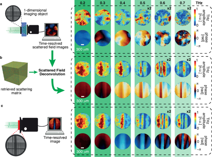
Hyperspectral image retrieval through scattering media. (a) Broadband scrambled field and phase profiles of a 1D imaging object (inset image: 200 \(\:\mu\:m\) thick copper wire over a reference ruler with ticks spaced 100 μm) hidden behind the scattering media (video 3). (b) Hyperspectral image retrieval: the data in a. are deconvoluted by the reconstructed transmission matrix of a scattering sample (video 4). (c) Hyperspectral THz images of the 1D imaging object used in a. for comparison (video 5).