Hybrid light-matter states, the polaritonic states, emerge in an optical cavity as the result of strong coupling between the cavity photon with the frequency ωc and molecular electronic states under the regime where the coherent energy exchange between them is faster than the energy dissipation29. When the light-matter coupling is absent, i.e., when the coupling strength g = 0, the combined states of the cavity photons and molecular electronic states are given as simple direct products \(\vert n,p\big\rangle=\vert n\big\rangle \otimes \vert p\big\rangle\), where n = S0, S1, … labels the molecular electronic states and p = 0, 1, … labels the states of p photons, see Fig. 2. Under the zero coupling, the diabatic (or uncoupled) states \(\vert {{{\rm{S}}}}_{0},0\big\rangle\) and \(\vert {{{\rm{S}}}}_{1},0\big\rangle\) are identical to the bare S0 and S1 states, and the \(\vert {{{\rm{S}}}}_{0},1\big\rangle\) and \(\vert {{{\rm{S}}}}_{1},1\big\rangle\) are replicas of the bare molecular states shifted upwards by the photon frequency ωc.
Fig. 2: Jablonski diagram of molecular energy levels under strong molecule-cavity coupling regime.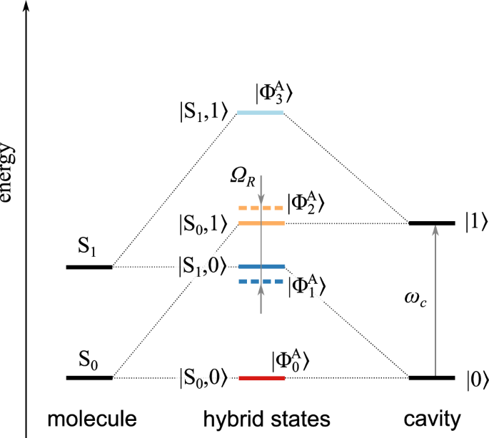
The polaritonic states emerge from the hybridization of the parent molecular electronic states with the photons with the frequency ωc. For hybrid states, the solid and dashed lines represent the diabatic (or uncoupled) and adiabatic (or polaritonic) states, respectively. The Rabi splitting ΩR is determined from the strength of the molecule-cavity coupling.
When the molecular-photon interaction is turned on, i.e., g ≠ 0 (by definition, \(g=\sqrt{\frac{\hbar {\omega }_{c}}{2{\epsilon }_{0}{V}_{c}}}\) where ωc is the cavity photon frequency, ϵ0 is the vacuum permittivity, and Vc is the effective mode volume of the cavity photon), the diabatic states closest in energy will mix and form new adiabatic polaritonic states \(\vert {\Phi }_{k}^{A}\big\rangle\) (k = 0, 1, 2, 3). Usually, the cavity eigenmode ωc is tuned to match the molecular vertical excitation energy, such that the \(\vert {{{\rm{S}}}}_{1},0\big\rangle\) and \(\vert {{{\rm{S}}}}_{0},1\big\rangle\) states become (nearly) degenerate and the adiabatic states \(\vert {\Phi }_{1}^{A}\big\rangle\) and \(\vert {\Phi }_{2}^{A}\big\rangle\) become their superpositions split by an energy gap known as the Rabi splitting ΩR (\({\Omega }_{R}=2{{\boldsymbol{\mu }}}\cdot {{\boldsymbol{\lambda }}}\sqrt{N}\hbar g\), where N is the number of molecules, μ is the transition dipole moment, and λ is a unit vector along the field polarization). The other two diabatic states, \(\vert {{{\rm{S}}}}_{0},0\big\rangle\) and \(\vert {{{\rm{S}}}}_{1},1\big\rangle\), remain unmodified because the interaction strength g is typically much smaller than the splitting between the bare energy levels.
Because the new \(\vert {\Phi }_{1}^{A}\big\rangle\) and \(\vert {\Phi }_{2}^{A}\big\rangle\) adiabatic states, also known as the lower (LP) and upper (UP) polaritonic states, are superpositions of the bare molecular \(\vert {{{\rm{S}}}}_{0}\big\rangle\) and \(\vert {{{\rm{S}}}}_{1}\big\rangle\) states, their potential energy surfaces (PESs) are strongly modified by the cavity-molecule interaction; especially in the regions where the diabatic \(\vert {{{\rm{S}}}}_{1},0\big\rangle\) and \(\vert {{{\rm{S}}}}_{0},1\big\rangle\) states were the closest in energy. The cavity-molecule interaction depends on the transition dipole moment between the S1 and S0 states (see the Methods section for details) and the modulation of molecular PESs becomes more pronounced in the geometries with large transition dipole.
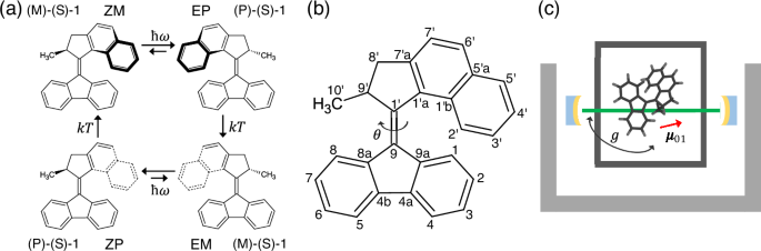
The outlined JC model was implemented in connection with the DFTB/SSR method as described in ref. 55 and the PESs and non-adiabatic molecular dynamics (NAMD) of the motor 1 were studied using the LC-OC-DFTB/SSR method55,56,57,58 (see the Methods section for detail). In the following, the analysis of the potential energy surfaces and dynamics will be presented for a zero field case (a free motor molecule outside the cavity), as well as for a few cases of cavity-molecule coupling, the resonant coupling and two off-resonant coupling scenarios, red-detuned and blue-detuned conditions38. In all cases, the forward, ZM → EP, and backward, EP → ZM, photoreactions are studied. The other two possible photoreactions in Fig. 1c (i.e., EM → ZP and ZP → EM) are identical with the former and involve the motor molecule rotated through 180° with respect to its original orientation. When reporting results of the simulations, the potential energy surfaces and trajectories are characterized in terms of two geometric parameters, the dihedral angle θ representing the torsion about the C9=\({{{\rm{C}}}}_{{1}^{{\prime} }}\) bond (see Fig. 1a) and the pyramidalization angle ϕ at the C9 atom59. First, the photoreactions will be investigated in the gas phase and a lossless optical cavity. Then, the effects of the environment and cavity losses will be simulated and analyzed. When simulating the effect of the environment, the possible interaction of the molecule with the metallic surface of the nanoplasmonic cavity is ignored. The use of a nanoplasmonic cavity is desirable for achieving magnitudes of the light-matter coupling strength sufficiently large for modifying the electronic states of the target molecule. The interaction with the cavity walls can be minimized by introducing insulating layers; to a certain degree, this can reduce the magnitude of the coupling with the cavity photons. These effects, however, are not considered here, and only the effect of the solvent present in the nanocavity is included.
Zero-coupling case in gas phase
As a reference for further comparisons, a zero-coupling (ZC, g = 0.0 a.u.) case was studied first in the gas phase; for solution phase calculations, see section “Effect of the environment”. The profiles of the potential energy surfaces (PESs) of the ground S0 and excited S1 states along the dihedral angle θ are shown in Fig. 3. The PES profiles were obtained by constraining the central dihedral angle and optimizing all other geometric parameters in the ground electronic state. The excited state energies were obtained from the single-point calculations in the respective geometries. The stable (ZM) structure is lower in energy than the metastable (EP) structure by 0.086 eV (1.98 kcal/mol), which is in reasonable agreement with 2.04 kcal/mol obtained previously by Pang et al. with the use of the semiempirical OM2/MRCI method in the gas phase60. In addition, two minima occur in the excited state, which are characterized by different dihedral angles θ, 283.4° in ZM(S1) and 254.3° in EP(S1); see Supplementary Fig. 1 for the optimized structures. Near the torsion angle θ ~ 270°, two S1/S0 conical intersections are located, which are characterized by opposite values of the pyramidalization angle ϕ, −16.7° in CI1 and +15.9° in CI2; see insets in Fig. 3. The occurrence of these conical intersections is consistent with the results of Pang et al.60 and with the previous theoretical works on a related molecular motor61,62.
Fig. 3: Profiles of the ground and excited PESs of the motor 1 along the dihedral angle θ in the absence of coupling with the cavity photon.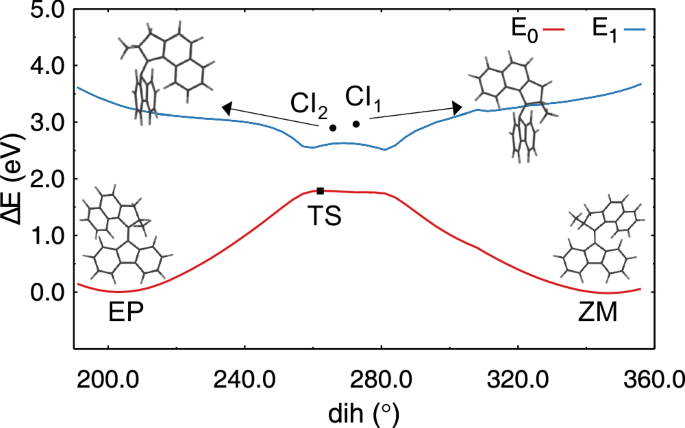
The relaxed scan was obtained by constraining the dihedral (dih) angle in the ground electronic state. The insets show the structures of the ground state minima (ZM and EP) and the minimum energy conical intersections (MECI), CI1 and CI2, between the S0 and S1 states occurring near the dihedral angle θ ~ 270°. The pyramidalization and dihedral angles (ϕ, θ) for the ZM, CI1, CI2, and EP structures are (−1.39°, 345.8°), (−16.7°, 272.6°), (15.9°, 265.8°), and (−1.36°, 202.6°), respectively. The values (ϕ, θ) for the transition state (TS) structure are (−1.40°, 262.1°). Source data are provided as a Source Data file.
In addition to constrained optimization, minimum energy path (MEP) optimizations were performed for the ZM → EP, and EP → ZM photoreactions, which are shown in Supplementary Fig. 2. Starting from the Franck-Condon point of ZM or EP structure on the S1 PES, the motor 1 approaches the S1 minimum through a barrierless pathway by changing the central dihedral angle θ. Further relaxation occurs via CI1 or CI2, characterized by substantial pyramidalization distortion. Both conical intersections are energetically accessible from the Franck-Condon point. After reaching a conical intersection, the photoisomerization reaction switches to the S0 state and completes the transformation along the dihedral angle degree of freedom. In addition, a transition state (TS) structure on the ground state PES was optimized (see Fig. 3 and Supplementary Fig. 3). For the motor 1, the homolytic breaking of the central π-bond is favorable in the S0 state, which results in the TS structure having the diradical (DIR) characteristics. In the S1 state, the TS structure acquires the charge transfer (CT) character. Therefore, the conical intersections are accessed by pyramidalization distortion, which connects the DIR and CT structures63. The relative energies of all optimized structures are given in Supplementary Table 1.
The NAMD trajectories were initiated in the geometries obtained by Boltzmann sampling of the ground state trajectories ran for 20 ps with a time step of 0.5 fs under the velocity-rescaling thermostat at 300 K. In total, 100 NAMD trajectories were started in these geometries by populating initially the S1 state and running the simulations for 5 ps with a time step of 0.5 fs under the NVE (or micro-canonical) ensemble conditions.
The resulting population dynamics during the ZM → EP and EP → ZM photoreactions are shown in Fig. 4. The average S1 state lifetimes for both photoreactions are 2.75 ps for ZM → EP and 2.21 ps for EP → ZM. The obtained S1 lifetime of the ZM → EP stage is considerably longer than ca. 710 fs obtained by Pang et al.60 in the semiempirical OM2/MRCI simulations, and agrees better with the experimental estimates. Thus, Conyard et al. obtained 1.5 ± 0.3 ps for the exponential decay constant of the S1 state that is populated a few hundred femtoseconds after the start of the ZM → EP photoreaction64. This suggests that the measured S1 lifetime may vary in the range of 1.7–2.1 ps, which is in reasonable agreement with the lifetimes obtained here.
Fig. 4: Time evolution of the populations of the electronic states in the zero-coupling case.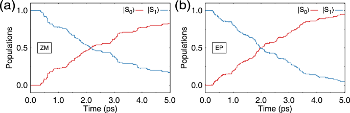
a Population dynamics during the ZM → EP photoreaction. The red and blue curves show populations of the S0 and S1 states, respectively. b Population dynamics during the EP → ZM photoreaction. Source data are provided as a Source Data file.
Out of a hundred trajectories started for the ZM → EP and EP → ZM photoreactions, 83 and 95 trajectories have undergone the S1 → S0 population transfer and the rest of the trajectories remained in the S1 state at the end of the simulations (5 ps). For the ZM → EP photoreaction, 40 trajectories reached the EP structure on the S0 PES, and 43 trajectories returned to the ZM structure, which corresponds to the quantum yield of 48.2%. This quantum yield (QY) is somewhat lower than 59.9% obtained by Pang et al. in their gas phase simulations60. The remaining difference with the experimental QY of 14%65 is likely to be caused by solvent because the solvent molecules in the solvation shell do not have sufficient time to rearrange during the ultrafast photoisomerization and mainly keep the arrangement that favors the solute structure at the beginning of the photoreaction66,67. The effect of the environment is discussed in the section “Effect of the environment” below. For the EP → ZM photoreaction, the respective QY is 41.1% (39 trajectories ended in ZM and 56 returned to EP), which is marginally lower than in the ZM → EP photoreaction. Overall, the obtained characteristics of the ZM → EP and EP → ZM photoreactions of 1 are consistent with previous theoretical simulations60.
Resonant strong coupling in gas-phase lossless optical cavity
Turning to non-zero coupling between the cavity mode and the molecule, the case of resonant coupling was studied first. For this case, the cavity mode frequency ωc was tuned to the energy of the vertical electronic transition of the starting structures of the ZM → EP and EP → ZM photoreactions in their equilibrium ground state geometries. Therefore, ħωc was set to 3.54 eV for the ZM structure and to 3.3 eV for the EP structure. The coupling strength g was set to 0.001 a.u. and the electric field of the cavity mode was set parallel to the central C9=\({{{\rm{C}}}}_{{1}^{{\prime} }}\) double bond. It is noteworthy that the transition dipole moment of the S1 ← S0 transition is almost perfectly parallel to the C9=\({{{\rm{C}}}}_{{1}^{{\prime} }}\) bond for both structures, ZM and EP (see Supplementary Fig. 4).
The profiles of the polaritonic PESs (PPESs) of the ZM → EP and EP → ZM photoreactions along the central dihedral angle θ are shown in Fig. 5. The geometries of the ground state equilibrium structures and the profile of the ground polaritonic state \(\vert {\Phi }_{0}^{A}\big\rangle\) remain in the SC case the same as in the ZC case. As seen in Fig. 2, the lowest polaritonic state \(\vert {\Phi }_{0}^{A}\big\rangle\) is unaffected by the cavity-molecule interaction, and the characteristics of this state are the same as the ground electronic state. The same is true for the highest polaritonic state \(\vert {\Phi }_{3}^{A}\big\rangle\), which replicates the profile of the uncoupled S1 electronic state, which is now dressed by a single cavity photon, and its energy is translated upwards by the photon frequency.
Fig. 5: Potential energy curves of the motor 1 strongly coupled to a single cavity.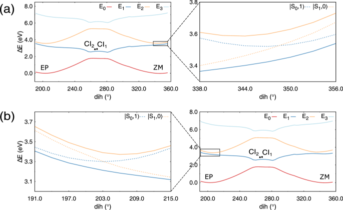
a Profiles of polaritonic states along the dihedral (dih) angle θ for the ZM → EP photoreaction. The relaxed scan was obtained by constraining the dihedral angle in the ground polaritonic state. The cavity mode frequency is tuned to the vertical excitation energy of the ZM structure, i.e., 3.54 eV. The black dots in the main plot show the positions of two conical intersections, CI1 and CI2, between the \(\vert {\Phi }_{0}^{A}\big\rangle\) and \(\vert {\Phi }_{1}^{A}\big\rangle\) polaritonic states. The values (ϕ, θ) of the pyramidalization and dihedral angles of the ZM, CI1, CI2, and EP structures are (−1.39°, 345.8°), (−18.0°, 267.8°), (16.2°, 265.2°), and (−1.36°, 202.6°), respectively. The rectangular region in the main plot is magnified in the inset next to it. The dotted lines in the inset show the uncoupled states; see Fig. 2 for more detail. b The same for the EP → ZM photoreaction. The cavity mode is tuned to 3.3 eV, which corresponds to the vertical excitation energy of the EP structure. The values (ϕ, θ) of the pyramidalization and dihedral angles of the EP, CI1, CI2, and ZM structures are (−1.36°, 202.6°), (−18.0°, 267.8°), (16.2°, 265.2°), and (−1.39°, 345.8°), respectively. Note that the same range of the central dihedral angle θ is chosen in panels (a) and (b); which means that the ZM structure corresponds to θ ≈ 360°. Source data are provided as a Source Data file.
The greatest alteration occurs for the lower polaritonic \(\vert {\Phi }_{1}^{A}\big\rangle\) and the upper polaritonic \(\vert {\Phi }_{2}^{A}\big\rangle\) states, which become superpositions of the uncoupled \(\vert {{{\rm{S}}}}_{0},1\big\rangle\) and \(\vert {{{\rm{S}}}}_{1},0\big\rangle\) states, i.e., \(\vert {\Phi }_{1}^{A}\big\rangle \sim \frac{1}{\sqrt{2}}\vert {{\mbox{S}}}_{0},1\big\rangle+\frac{1}{\sqrt{2}}\vert {{\mbox{S}}}_{1},0\big\rangle\) and \(\vert {\Phi }_{2}^{A}\big\rangle \sim \frac{1}{\sqrt{2}}\vert {{\mbox{S}}}_{0},1\big\rangle -\frac{1}{\sqrt{2}}\vert {{\mbox{S}}}_{1},0\big\rangle\), split due to the cavity-molecule interaction. The Rabi splitting ΩR between the \(\vert {\Phi }_{1}^{A}\big\rangle\) and \(\vert {\Phi }_{2}^{A}\big\rangle\) states becomes 173 and 178 meV for the ZM and EP equilibrium structures, respectively. This corresponds to ΩR on the order of a few percent (ca. 5%) of the vertical excitation energy of the motor, which is typical for the strong coupling regime. Note that, ΩR exceeding ca. 20% of the molecular excitation energy implies the ultrastrong coupling regime, which is not addressed in this paper.
Although a noticeable modulation of the potential energy surfaces is seen near the ground state equilibrium geometries of the ZM and EP structures, no new local minima or transition states emerge on these surfaces. This implies that the dynamics of the motor in the resonant SC regime may not be very strongly affected by the cavity-molecule interaction. To verify this conjecture, a series of NAMD simulations have been carried out for the resonant SC regime. In these simulations, the same initial geometries as in the ZC case were used. In total, 100 trajectories were propagated for each photoreaction, ZM → EP and EP → ZM. At the beginning of the trajectories, the upper polaritonic state \(\vert {\Phi }_{2}^{A}\big\rangle\) was populated, and the trajectories were propagated up to 5 ps with a timestep of 0.5 fs.
The population dynamics obtained for both photoreactions are shown in Fig. 6. In both photoreactions, the upper polaritonic state \(\vert {\Phi }_{2}^{A}\big\rangle\) is rapidly (within less than 100 fs) depopulated, and its population is transferred to the lower polaritonic state \(\vert {\Phi }_{1}^{A}\big\rangle\). The \(\vert {\Phi }_{2}^{A}\big\rangle \to \vert {\Phi }_{1}^{A}\big\rangle\) decay begins immediately upon excitation and occurs with the decay constants of 42.7 and 35.7 fs for the ZM → EP and EP → ZM reactions, respectively. Upon the rapid initial population transfer, the \(\vert {\Phi }_{1}^{A}\big\rangle\) state begins to slowly decay to the ground polaritonic state \(\vert {\Phi }_{0}^{A}\big\rangle\), with a latency time of ca. 200–300 fs for both photoreactions. Analysis of the populations of the electronic states (see Supplementary Fig. 5) reveals that, at the beginning of the photoreaction, both electronic states S1 and S0 are equally populated due to the entanglement in the polaritonic states \(\vert {\Phi }_{2}^{A}\big\rangle\) and \(\vert {\Phi }_{1}^{A}\big\rangle\). The \(\vert {\Phi }_{2}^{A}\big\rangle \to \vert {\Phi }_{1}^{A}\big\rangle\) decay results in a disentanglement of the electronic states, and the S1 state becomes nearly fully populated within the first ca. 200–300 fs. Then, the S1 population begins to decay to the ground electronic state due to the \(\vert {\Phi }_{1}^{A}\big\rangle \to \vert {\Phi }_{0}^{A}\big\rangle\) transfer. The \(\vert {\Phi }_{1}^{A}\big\rangle \to \vert {\Phi }_{0}^{A}\big\rangle\) population transfer follows exponential decay, with the lifetimes of 2.50 ps and 2.66 ps for the ZM → EP and EP → ZM reactions, respectively.
Fig. 6: Time evolution of the populations of the polaritonic states in the resonant strong coupling case.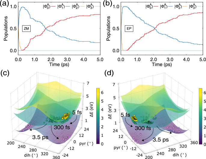
a Population dynamics during the ZM → EP photoreaction. b Population dynamics during the EP → ZM photoreaction. c Location of the ZM → EP trajectories at specific instances of time shown on scanned surfaces of the upper polaritonic (yellowish colours) \(\vert {\Phi }_{2}^{A}\big\rangle\) state, lower polaritonic (greenish colours) \(\vert {\Phi }_{1}^{A}\big\rangle\) state, and the ground polaritonic (purplish colours) \(\vert {\Phi }_{0}^{A}\big\rangle\) state with respect to the dihedral (dih) and pyramidalization (pyr) angles. The squares show trajectory points at 5 fs, the triangles at 300 fs, and the circles at 3.5 ps propagation time. The yellow markers show trajectories residing in the \(\vert {\Phi }_{2}^{A}\big\rangle\) state, the green markers show trajectories in the \(\vert {\Phi }_{1}^{A}\big\rangle\) state, and the purple markers the trajectories in the \(\vert {\Phi }_{0}^{A}\big\rangle\) state. d The same for the EP → ZM photoreaction. Source data are provided as a Source Data file.
The latency in the \(\vert {\Phi }_{1}^{A}\big\rangle \to \vert {\Phi }_{0}^{A}\big\rangle\) decay is caused by the necessity for the nuclear trajectories to reach structures in geometrical proximity of the \(\vert {\Phi }_{1}^{A}\big\rangle\)/\(\vert {\Phi }_{0}^{A}\big\rangle\) conical intersections, which occur at the torsion angle θ near ca. 270°; see Fig. 5. Analysis of the geometries along the trajectories suggests that this occurs after approximately 700 fs since the start of the trajectories. By this time, the majority of trajectories reach the minimum on the \(\vert {\Phi }_{1}^{A}\big\rangle\) PPES (see Fig. 6) and remain in its basin, slowly decaying to the \(\vert {\Phi }_{0}^{A}\big\rangle\) state through the CI1 and CI2 intersections. Supplementary Fig. 6 shows a distribution of the number of trajectories approaching CI1 or CI2 at different instances of time. The majority of trajectories decay through CI2, however (quasi-)periodic oscillations with a period of ≈ 1.0 ps are observed for the decay events through CI2 and CI1; see Supplementary Fig. 6. The relatively long period of oscillations between decays through CI2 and CI1 is caused by large variations in the pyramidalization angle needed to reach the respective CI seams. Similar oscillations caused by the wobbling of the central double bond during the dynamics have also been noticed in the previous NAMD simulations61. It is noteworthy that, during the dynamics, the orientation of the central C=C double bond on average remains the same as at the beginning of the photoreaction. This happens because the coupling with the cavity photon’s electric field exerts a relatively low net force on the motor 1, which remains predominantly aligned with the C=C bond direction. As seen in Supplementary Fig. 7, the polaritonic PESs remain essentially flat along the alignment angle, defined as the angle between the C=C bond and the cavity axis (see Fig. 1c).
During the 5 ps propagation time, 82 trajectories in the ZM → EP reaction and 87 trajectories in the EP → ZM reaction undergo the \(\vert {\Phi }_{1}^{A}\big\rangle \to \vert {\Phi }_{0}^{A}\big\rangle\) population transfer. In the ZM → EP reaction, 50 trajectories move forward and produce the EP final structure and 32 trajectories turn back towards the ZM structure. The ratio of the productive to unproductive trajectories changes to 48:39 in the EP → ZM reaction. Therefore, the two photoreactions exhibit quantum yields of 61.0% (ZM → EP) and 55.2% (EP → ZM), which are not much different from the zero-field scenario; 48.2% and 41.1%, respectively. Given that the lifetimes of the \(\vert {\Phi }_{1}^{A}\big\rangle \to \vert {\Phi }_{0}^{A}\big\rangle\) decay in the resonant SC case are almost the same as in the field-free case, we can conclude that the resonant coupling with a cavity mode does not considerably alter the characteristics of the ZM → EP and EP → ZM photoreactions.
JC model versus quantum Rabi model
So far the JC model has been used in our work, which uses the (low-frequency) rotating-wave approximation and neglects the effect of the (high-frequency) counter-rotating contribution. To evaluate the effect of the rotating-wave approximation, the potential energy surfaces and photodynamics of the two photoreactions of the motor 1 have been investigated with the use of the full quantum Rabi model, which includes the counter-rotating contributions; see the Methods section. The inclusion of the counter-rotating terms leads to coupling between the \(\vert {{\mbox{S}}}_{0},0\big\rangle\) and \(\vert {{\mbox{S}}}_{1},1\big\rangle\) diabatic states in the lowest polaritonic \(\vert {\Phi }_{0}^{A}\big\rangle\) and highest polaritonic \(\vert {\Phi }_{3}^{A}\big\rangle\) states. However, because the energy gap between the diabatic states is sufficiently wide, this results in only minor alteration of the dynamics and potential energy surfaces of the motor 1. The profiles of the PPESs of the ZM → EP and EP → ZM photoreactions along the central dihedral angle θ are shown in Supplementary Fig. 8. The new \(\vert {\Phi }_{0}^{A}\big\rangle\) and \(\vert {\Phi }_{3}^{A}\big\rangle\) states are strongly dominated by the \(\vert {{\mbox{S}}}_{0},0\big\rangle\) and \(\vert {{\mbox{S}}}_{1},1\big\rangle\) diabatic states, respectively, which remain effectively uncoupled. Compared to the JC model (which neglects the counter-rotating term), similar equilibrium structures of the \(\vert {\Phi }_{0}^{A}\big\rangle\) state and CIs between the \(\vert {\Phi }_{0}^{A}\big\rangle\) and \(\vert {\Phi }_{1}^{A}\big\rangle\) states are obtained in the quantum Rabi model.
In addition to studying the potential energy surfaces, 50 NAMD trajectories for both photoreactions were propagated for the Rabi model. Because the cavity-molecule interaction does not largely affect the lowest polaritonic \(\vert {\Phi }_{0}^{A}\big\rangle\) state, the same initial sampling conditions as in the ZC case were used. The population dynamics obtained for both photoreactions are shown in Supplementary Fig. 9. The characteristics of both photoreactions with the use of the Rabi model are nearly the same as with the use of the JC model: The \(\vert {\Phi }_{2}^{A}\big\rangle \to \vert {\Phi }_{1}^{A}\big\rangle\) decay occurs with the decay constants of 52.0 and 32.9 fs for the ZM → EP and EP → ZM reactions, respectively. After the initial population transfer, the \(\vert {\Phi }_{1}^{A}\big\rangle\) state decays to the lowest polaritonic \(\vert {\Phi }_{0}^{A}\big\rangle\) state, with the lifetimes of 2.36 and 2.84 ps for the ZM → EP and EP → ZM reactions, respectively. During the 5 ps propagation time, 44 trajectories in the ZM → EP reaction and 46 trajectories in the EP → ZM reaction undergo the \(\vert {\Phi }_{1}^{A}\big\rangle \to \vert {\Phi }_{0}^{A}\big\rangle\) population transfer. In the former case, 26 trajectories reach the final EP structure and 18 trajectories turn back towards the ZM structure. The ratio of the productive to unproductive trajectories changes to 21:25 in the EP → ZM reaction. Therefore, the quantum yields of 59.1% and 45.7% for the two photoreactions are obtained, which are close to both the ZC case (48.2% and 41.1%) and to the SC case with the JC model (61.0% and 55.2%). This implies that the rotating-wave approximation used in the JC model is sufficiently accurate for our simulations and will be used in the rest of the work.
Off-resonant strong coupling case
The resonant SC scenario studied above results in a strong mixing between the \(\vert {{\mbox{S}}}_{0},1\big\rangle\) and \(\vert {{\mbox{S}}}_{1},0\big\rangle\) diabatic states in the upper and lower polaritonic states near the ground state equilibrium geometry of both structures, ZM and EP. Therefore, the lower polaritonic state \(\vert {\Phi }_{1}^{A}\big\rangle\) retains the most prominent characteristics of the \(\vert {{\mbox{S}}}_{1},0\big\rangle\) diabatic state, which has a pronounced slope in the direction of torsion about the central dihedral angle θ; see Fig. 5. Because the \(\vert {\Phi }_{2}^{A}\big\rangle \to \vert {\Phi }_{1}^{A}\big\rangle\) population transfer occurs on an ultrafast timescale (less than ca. 50 fs) and is not accompanied by a noticeable change of the angle θ, the dynamics of the LP state \(\vert {\Phi }_{1}^{A}\big\rangle\) begins on a surface strongly resembling the \(\vert {{\mbox{S}}}_{1},0\big\rangle\) PES. As a consequence, with the resonant excitation, the dynamics of the \(\vert {\Phi }_{1}^{A}\big\rangle \to \vert {\Phi }_{0}^{A}\big\rangle\) decay shows characteristics very similar to the field-free (ZC) case; see Fig. 4.
Here, we would like to inspect whether detuning the cavity mode frequency off-resonance with the molecular vertical transition can result in a stronger modification of the polaritonic PESs and the ensuing dynamics. To address this question, we have undertaken a series of NAMD simulations with the cavity mode frequency ωc red-detuned and blue-detuned by 1.0 eV off-resonance with the respective molecular vertical excitation energy. In the case of the ZM → EP photoreaction, this implies using ωc of 2.54 (red-detuned) and 4.54 eV (blue-detuned), and for the EP → ZM photoreaction the ωc values of 2.3 and 4.3 eV, respectively. The coupling strength g in all cases was kept at its value used in the resonant SC case; i.e., 0.001 a.u. All simulations with the off-resonant frequencies begin in the upper polaritonic state.
Figure 7 shows the results for the ZM → EP photoreaction, where the upper polaritonic state was populated at the start. In the red-detuned case (ωc = 2.54 eV), the mixing between the \(\vert {{\mbox{S}}}_{0},1\big\rangle\) and \(\vert {{\mbox{S}}}_{1},0\big\rangle\) diabatic states occurs in a region of the dihedral angle θ shifted ca. 35° away from the Franck-Condon (FC) region; see Fig. 7a. Near the FC geometry, the LP state \(\vert {\Phi }_{1}^{A}\big\rangle\) is almost entirely equivalent to the \(\vert {{\mbox{S}}}_{0},1\big\rangle\) diabatic state and there is a local minimum near θ ≈ 346° (or −14°) separated from the local minima at ca. ~270° (or −90°) by a barrier, seen in Fig. 7a. A similar shape of the PPES profile is seen in Fig. 7a for the values of θ approaching the EP structure (θ \(\vert {\Phi }_{2}^{A}\big\rangle \to \vert {\Phi }_{1}^{A}\big\rangle\) population transfer, a substantial part of the population can be diverted toward the new local minimum and will remain in the \(\vert {\Phi }_{1}^{A}\big\rangle\) polaritonic state for a prolonged time; thus, essentially, blocking isomerization of ZM to EP.
Fig. 7: Potential energy surfaces and non-adiabatic population dynamics of the ZM → EP photoreaction in the off-resonant strong coupling case.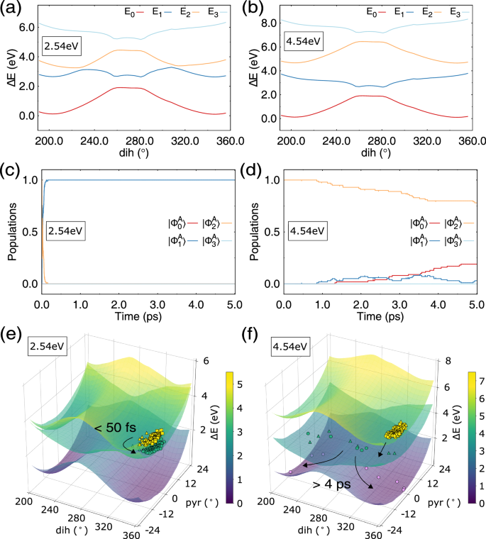
a Polaritonic potential energy curves with respect to the dihedral angle θ and c time evolution of the populations of the polaritonic states for ωc = 2.54 eV. The relaxed scan was obtained by constraining the dihedral angle in the ground polaritonic state. e Location of the trajectories (ωc = 2.54 eV) at specific instances of time shown on scanned surfaces of the upper polaritonic (yellowish colours) \(\vert {\Phi }_{2}^{A}\big\rangle\) state, lower polaritonic (greenish colours) \(\vert {\Phi }_{1}^{A}\big\rangle\) state, and the ground polaritonic (purplish colours) \(\vert {\Phi }_{0}^{A}\big\rangle\) state with respect to the dihedral (dih) and pyramidalization (pyr) angles. The squares show trajectory points at 5 fs, the triangles at 50 fs, and the circles at 2.4 ps propagation time. The yellow markers show trajectories residing in the \(\vert {\Phi }_{2}^{A}\big\rangle\) state, the green markers show trajectories in the \(\vert {\Phi }_{1}^{A}\big\rangle\) state, and the purple markers the trajectories in the \(\vert {\Phi }_{0}^{A}\big\rangle\) state. b, d, and f The same for the cavity mode frequency ωc = 4.54 eV. The square, triangular, and circular markers in panel f show trajectory points at 5 fs, 2.0 ps, and 4.0 ps, respectively. Source data are provided as a Source Data file.
To verify this conjecture, we ran a series of NAMD simulations, which were set up in the same way as in the resonant SC case, with the sole difference that ωc was now set to 2.54 eV. The time evolution of the polaritonic state populations is shown in Fig. 7c. As seen in the figure, the initial \(\vert {\Phi }_{2}^{A}\big\rangle\) population is transferred to \(\vert {\Phi }_{1}^{A}\big\rangle\) on an ultrafast timescale with a lifetime of 32.9 fs. Although at the start of the trajectories, the UP state is dominated by the S1 contribution and the LP state by the S0 contribution, the two polaritonic states very rapidly (~10 fs) become superpositions of the S1 and S0 electronic states, which become equally populated; see Supplementary Fig. 10a. The \(\vert {\Phi }_{2}^{A}\big\rangle \to \vert {\Phi }_{1}^{A}\big\rangle\) population transfer results in a rapid decay of the S1 population, which is transferred to the S0 state. After that, for the whole duration of the simulations (5 ps), the populations remain in the \(\vert {\Phi }_{1}^{A}\big\rangle\) state, which is dominated by the S0 electronic state, and no rotation about the central double bond takes place. Therefore, an off-resonant red-detuning of the cavity mode has the potential to block the isomerization of the motor and its rotation.
In addition to simulations started in the upper polaritonic state \(\vert {\Phi }_{2}^{A}\big\rangle\), a series of simulations where the lower polaritonic state \(\vert {\Phi }_{1}^{A}\big\rangle\) was initially populated have been carried out. As shown in Supplementary Fig. 11, the change in the initial state does not lead to significant changes in the dynamics; the rotation of the motor 1 remains blocked due to the off-resonant red-detuned coupling.
A different picture of the dynamics is observed in the blue-detuned case (ωc = 4.54 eV); see Fig. 7b, d, and f. The \(\vert {{\mbox{S}}}_{0},1\big\rangle\) diabatic state is shifted upwards considerably above the \(\vert {{\mbox{S}}}_{1},0\big\rangle\) diabatic state, which effectively minimizes their mixing in the UP and LP states; see Fig. 7b. Consequently, when populating the \(\vert {\Phi }_{2}^{A}\big\rangle\) state at the beginning of the simulations, where trajectories are localized in the well near ZM configuration due to the strong S0 contribution (see also Supplementary Fig. 10b), very slow decay of its population ensues on a timescale much longer than the simulation time (5 ps); mainly due to the finite energy gap between the UP and LP states. Within the simulation time, only 22 trajectories (out of 100) undergo the \(\vert {\Phi }_{2}^{A}\big\rangle \to \vert {\Phi }_{1}^{A}\big\rangle\) population transfer (78 remain in \(\vert {\Phi }_{2}^{A}\big\rangle\)), out of which 19 trajectories subsequently undergo population transfer to the ground \(\vert {\Phi }_{0}^{A}\big\rangle\) polaritonic state and 3 remain in the \(\vert {\Phi }_{1}^{A}\big\rangle\) state. The \(\vert {\Phi }_{1}^{A}\big\rangle \to \vert {\Phi }_{0}^{A}\big\rangle\) transfer occurs essentially on the same timescale as in the field-free case because the \(\vert {\Phi }_{1}^{A}\big\rangle\) polaritonic state is almost pure S1 electronic state and \(\vert {\Phi }_{0}^{A}\big\rangle\) is S0 (see Supplementary Fig. 10b). As seen in Fig. 7d, the depletion of the \(\vert {\Phi }_{2}^{A}\big\rangle\) population is comparable to the recovery of the \(\vert {\Phi }_{0}^{A}\big\rangle\) population, accompanied by an intermittent population of the \(\vert {\Phi }_{1}^{A}\big\rangle\) state. In the end, 10 trajectories reach the EP structure and 9 fall back to the ZM structure; which produces a quantum yield (52.6%) very close to the field-free case (48.2%). Although there is no complete blockade of the rotation as in the red-detuning case, the blue-detuning has the potential to slow down the photoisomerization process without strongly affecting its quantum yield.
In addition to simulations started in the upper polaritonic state, a series of simulations initiated in the lower polaritonic state have been carried out. Because the lower polaritonic state \(\vert {\Phi }_{1}^{A}\big\rangle\) remains almost pure S1 state, the dynamics typical for the field-free situation has been observed; see Supplementary Fig. 12. Therefore, in the blue-detuned scenario, the dynamics is strongly affected by the initial population of the polaritonic states.
Generally, a quite similar picture is observed in the off-resonant coupling simulations of the EP → ZM photoreaction; see Fig. 8. In the red-detuned case (ωc = 2.3 eV), the barrier on the \(\vert {\Phi }_{1}^{A}\big\rangle\) PPES occurs at ca. 233° of torsion, near which the \(\vert {{\mbox{S}}}_{0},1\big\rangle\) and \(\vert {{\mbox{S}}}_{1},0\big\rangle\) diabatic states are strongly mixed; see Fig. 8a and Supplementary Fig. 10c. When starting in the fully populated \(\vert {\Phi }_{2}^{A}\big\rangle\) state, the population evolves as shown in Fig. 8c, where it is seen that population transfer to the \(\vert {\Phi }_{1}^{A}\big\rangle\) state occurs on a very rapid timescale of 21.8 fs. As shown in Supplementary Fig. 10c, this results in redistribution of the populations of the S1 and S0 electronic states, very similar to what was observed for the ZM → EP photoreaction. Upon the \(\vert {\Phi }_{2}^{A}\big\rangle \to \vert {\Phi }_{1}^{A}\big\rangle\) transfer, the \(\vert {\Phi }_{1}^{A}\big\rangle\) population decays on an extremely slow timescale, where only three trajectories undergo a transition to the ground state until the end of the simulations. Out of the three trajectories, two move forward to the ZM structure and one falls back to EP; which produces a (not statistically meaningful) quantum yield of 66.6%. Given that only three trajectories underwent transition to the ground state, it is very difficult to estimate the possible excited state lifetime in this case. However, it is plausible that the motor’s rotation is blocked for a prolonged time.
Fig. 8: Potential energy surfaces and non-adiabatic population dynamics of the EP → ZM photoreaction in the off-resonant strong coupling case.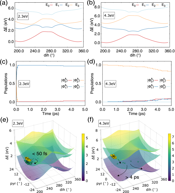
a Polaritonic potential energy curves with respect to the dihedral angle θ and c time evolution of the populations of the polaritonic states for ωc = 2.3 eV. The relaxed scan was obtained by constraining the dihedral angle in the ground polaritonic state. e Location of the trajectories (ωc = 2.3 eV) at specific instances of time shown on scanned surfaces of the upper polaritonic (yellowish colours) \(\vert {\Phi }_{2}^{A}\big\rangle\) state, lower polaritonic (greenish colours) \(\vert {\Phi }_{1}^{A}\big\rangle\) state, and the ground polaritonic (purplish colours) \(\vert {\Phi }_{0}^{A}\big\rangle\) state with respect to the dihedral (dih) and pyramidalization (pyr) angles. The squares show trajectory points at 5 fs, the triangles at 50 fs, and the circles at 2.4 ps propagation time. The yellow markers show trajectories residing in the \(\vert {\Phi }_{2}^{A}\big\rangle\) state, the green markers show trajectories in the \(\vert {\Phi }_{1}^{A}\big\rangle\) state, and the purple markers the trajectories in the \(\vert {\Phi }_{0}^{A}\big\rangle\) state. b, d, and f The same for the cavity mode frequency ωc = 4.3 eV. The square, triangular, and circular markers in panel f show trajectory points at 5 fs, 2.0 ps, and 4.0 ps, respectively. Source data are provided as a Source Data file.
The blue-detuned dynamics (ωc = 4.3 eV) during the EP → ZM photoreaction is, generally, similar to the ZM → EP case; see Fig. 8b, d, and f. The blue-detuning results in the UP and LP states, which are represented by nearly pure \(\vert {{\mbox{S}}}_{0},1\big\rangle\) and \(\vert {{\mbox{S}}}_{1},0\big\rangle\) diabatic states, see Fig. 8b and Supplementary Fig. 10d, and the dynamics shows characteristics very similar to the dynamics of the blue-detuned ZM → EP photoreaction. During the simulation time, 17 trajectories undergo population transfer to the \(\vert {\Phi }_{1}^{A}\big\rangle\) state (83 remain in \(\vert {\Phi }_{2}^{A}\big\rangle\)), out of which nine trajectories go through to \(\vert {\Phi }_{0}^{A}\big\rangle\); see Fig. 8d. Out of nine decayed trajectories, seven move forward to the ZM structure and two fall back to EP. Because the number of trajectories is too small, no meaningful comparison of the quantum yield of this reaction can be made. However, as in the ZM → EP case, one might expect that much longer simulations would produce a quantum yield in close agreement with the field-free case. Therefore, it can be conjectured that similar to the ZM → EP case, blue-detuning offers a means to flexibly adjust the excited state lifetime (hence, the speed of the motor’s rotation) without strongly affecting the isomerization quantum yield.
Effect of the environment
So far, the simulations of the motor’s dynamics were carried out in the gas phase. Although gas-phase optical cavities have recently emerged68,69, the most widely used optical and plasmonic cavities are implemented in the condensed phase32,33,34,35,36,37,38. Therefore, it appears important to investigate the effect of the condensed-phase environment on the dynamics of the motor embedded in a cavity. Here, we follow the same logic as in the preceding sections and present the ZC, resonant SC, and off-resonant SC cases in a solvent (dichloromethane, DCM).
In ZC case, the dynamics of the motor 1 in the DCM solvent has been modeled by using the multiscale QM/MM approach, where the solute molecule is treated quantum mechanically and the solvent is described by an atomistic force field (see the Methods section for details). Because the experimental measurements on the motor 1 have been carried out in DCM solution, the same solvent is used in our simulations. The initial conditions for the QM/MM NAMD simulations have been prepared similarly to the gas-phase case, i.e., from Boltzmann sampling of the ground state trajectories running at 300 K for 30 ps with a time step of 0.5 fs under the velocity-rescaling thermostat. Using the initial sampling conditions, 50 NAMD trajectories have been propagated by populating initially the S1 state and running for 6 ps with a time step of 0.5 fs under the NVE ensemble conditions.
Figure 9 shows the population dynamics for ZM → EP and EP → ZM photoreactions occurring in DCM solvent. Compared to the gas-phase simulations, the lifetime of the S1 state becomes considerably longer than in the gas-phase simulations; it elongates from 2.75 ps and 2.21 ps for the ZM → EP and EP → ZM photoreactions, respectively, to 7.01 ps and 5.55 ps. The latter values were obtained by a monoexponential fit of the population curves and, because the population dynamics in Fig. 9 shows obvious non-exponential evolution, may be less precise than in the gas-phase case. Our main focus, however, is on the quantum yield of the two photoreactions, which becomes markedly lower than in the gas-phase simulations. The QYs for the ZM → EP and EP → ZM photoreactions obtained in DCM solvent are 25.0% and 38.9%, respectively, and are in reasonable agreement with the experimental QYs of 14.0% and 50.0%65. The QY for EP → ZM is larger than for ZM → EP, which is consistent with the experimental observation. Although a relatively small number of trajectories (50) were propagated in our simulations, which may increase the margin of error for the obtained averages, it seems that the QM/MM simulations are capable of reasonably reproducing the experimental results reported in ref. 65.
Fig. 9: Time evolution of the populations of the electronic states in the presence of DCM solvent in the zero-coupling case.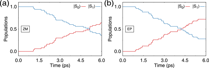
a Population dynamics during the ZM → EP photoreaction. The red and blue curves show populations of the S0 and S1 states, respectively. b Population dynamics during the EP → ZM photoreaction. Source data are provided as a Source Data file.
To investigate the effect of the environment in an optical cavity on the characteristics of the photodynamics of the motor 1 in resonant SC case, a series of QM/MM NAMD simulations in DCM have been carried out. Although the actual environment in a cavity may be different, our main purpose is to find out whether the general conclusions drawn from the gas-phase simulations still hold in a condensed-phase setting. For the cavity mode frequency ωc in resonance with the molecular vertical transitions, the same parameters as in the gas-phase simulations were used for the photon-molecule interaction. The initial conditions and the duration of the simulations are the same as in the field-free QM/MM simulations. The trajectories were started in the upper polaritonic state \(\vert {\Phi }_{2}^{A}\big\rangle\) fully populated. Supplementary Fig. 13 shows the population dynamics for both photoreactions obtained in DCM solvent. Similar to the gas-phase resonant SC regime, the \(\vert {\Phi }_{2}^{A}\big\rangle \to \vert {\Phi }_{1}^{A}\big\rangle\) decay is very rapid and occurs with the exponential decay constants of 51.5 and 81.3 fs for the ZM → EP and EP → ZM reactions, respectively. Upon the initial decay, the \(\vert {\Phi }_{1}^{A}\big\rangle\) state slowly decays to the ground \(\vert {\Phi }_{0}^{A}\big\rangle\) polaritonic state, with a latency time of ca. 500–700 fs for both photoreactions. The \(\vert {\Phi }_{1}^{A}\big\rangle \to \vert {\Phi }_{0}^{A}\big\rangle\) population transfer follows exponential decay with the lifetimes of 5.29 and 4.41 ps for the ZM → EP and EP → ZM reactions, respectively, which are slightly faster than in the ZC case. During the 6 ps propagation time, 36 trajectories in the ZM → EP reaction and 39 trajectories in the EP → ZM reaction undergo the \(\vert {\Phi }_{1}^{A}\big\rangle \to \vert {\Phi }_{0}^{A}\big\rangle\) population transfer, showing that the QYs are 22.2% and 30.8% for ZM → EP and EP → ZM reactions, respectively. Overall, the characteristics of the two photoreactions in the resonant SC regime do not differ substantially from the ZC case in the DCM solvent.
Similar to the gas-phase simulations, the red-detuned and blue-detuned scenarios were used for modeling the off-resonant strong molecule-cavity coupling. The population dynamics for the two scenarios is shown in Supplementary Fig. 14 for both photoreactions. In the red-detuned case, with ωc = 2.54 or 2.3 eV for the ZM → EP and EP → ZM photoreactions, the initial \(\vert {\Phi }_{2}^{A}\big\rangle\) population is transferred to \(\vert {\Phi }_{1}^{A}\big\rangle\) with lifetimes of 29.6 and 32.7 fs, which is close to the gas-phase simulations. After the initial population transfer, the population of the \(\vert {\Phi }_{1}^{A}\big\rangle\) state remains unchanged during the whole simulation time (6 ps), which implies that the isomerization of the motor 1 and its rotation is blocked by an off-resonant red-detuning of the cavity mode. In the off-resonant blue-detuned case, the QM/MM NAMD simulations predict that the initially populated \(\vert {\Phi }_{2}^{A}\big\rangle\) state decays very slowly to the lower polaritonic \(\vert {\Phi }_{1}^{A}\big\rangle\) state. The slow decay is caused by a wide gap between the UP and LP states. Within the simulation time (6 ps), out of 50 trajectories, only 4 trajectories in the ZM → EP reaction and 11 trajectories in the EP → ZM reaction undergo the \(\vert {\Phi }_{2}^{A}\big\rangle \to \vert {\Phi }_{1}^{A}\big\rangle\) population transfer. Upon decaying to the \(\vert {\Phi }_{1}^{A}\big\rangle\) state, the population transfer to the ground \(\vert {\Phi }_{0}^{A}\big\rangle\) state occurs on a timescale similar to the field-free scenario. Overall, as in the resonant case, the characteristics of the ZM → EP and EP → ZM photoreactions obtained in the condensed-phase simulations are very similar to the gas-phase case, and the major conclusions drawn from the latter results remain unchanged.
Photoisomerization reaction with cavity losses
The results presented so far were obtained in a lossless cavity, and they do not take into account the possibility of photon loss in the cavity. While long cavity photon lifetimes were obtained within high-quality and gas-phase microcavities,68,69,70 thus far mainly lossy plasmonic and optical microcavities have been used to achieve strong coupling with a single molecule36,71. Depending on the experimental setup, the photon lifetime in lossy cavities varies from a few dozen femtoseconds to nanoseconds,72,73,74,75,76,77,78,79 and it seems important to include the effect of photon disappearance on the obtained dynamics.
Here, we investigate the effect of photon loss on the gas-phase dynamics of the polaritonic states using a Monte Carlo approach (see Methods section)42,43. In the following, the photodynamics of the motor 1 was analyzed using three different values for the photon lifetime: 10, 100, and 2000 fs. In particular, we examine whether the retardation of dynamics observed in the simulations in a lossless cavity holds in the case of photon loss. The major finding is that irrespective of the photon lifetime, the inhibition of the motor’s rotation by resonant and off-resonant couplings takes place also in a lossy cavity.
In the case of strong resonant coupling, 100 gas-phase trajectories were replicated 10 times and post-processed for each lifetime, as described in the Methods section. Supplementary Figs. 15 and 16 show the population dynamics for both photoreactions, ZM → EP and EP → ZM, with cavity losses included, while Supplementary Fig. 17 represents the population projected on the electronic states S0 and S1. For the 2 ps photon lifetime, characteristics similar to a lossless cavity have been obtained for both photoreactions. In the case of 100 fs photon lifetime, the population of the lower polaritonic state \(\vert {\Phi }_{1}^{A}\big\rangle\) decreases markedly compared to the lossless case. The upper polaritonic to lower polaritonic state population transfer occurs on a faster timescale (≲50 fs) and is not responsible for the depletion of the \(\vert {\Phi }_{1}^{A}\big\rangle\) population. The latter depletion occurs due to a rapid loss of contribution from the \(\vert {{\mbox{S}}}_{0},1\big\rangle\) diabatic state and collapse to the \(\vert {{\mbox{S}}}_{0},0\big\rangle\) state as the result of photon disappearance. As a consequence, the population of the S0 electronic state rises rapidly, as seen in Supplementary Fig. 17c and d. Furthermore, the QY of isomerization decreases to 43.3% and 40.0% for the ZM → EP and EP → ZM photoreactions, respectively. With the shortest (10 fs) photon lifetime, the population of the \(\vert {\Phi }_{1}^{A}\big\rangle\) polaritonic state decreases even further, and the isomerization QY drops to 12.4% and 13.0% for the two photoreactions. Simultaneously with that, the ground state recovery time becomes noticeably faster, ≲1 ps; see Supplementary Figs. 15d and 16d. Therefore, there is a modulation of the motor’s photodynamics in the resonant coupling case, mainly manifested in the decreasing quantum yield of photoisomerization.
In the resonant SC case, the influence of cavity losses on the dynamics of motor 1 isomerization is relatively modest due to the short lifetime of the upper polaritonic \(\vert {\Phi }_{2}^{A}\big\rangle\) state. However, under strong off-resonant coupling conditions, the motor 1 remains for a prolonged time either in the \(\vert {\Phi }_{1}^{A}\big\rangle\) state (red-detuned scenario) or in the \(\vert {\Phi }_{2}^{A}\big\rangle\) state (blue-detuned scenario). In both situations, cavity losses can affect the dynamics, mainly due to the loss of the \(\vert {{\mbox{S}}}_{0},1\big\rangle\) contribution in the polaritonic states and collapse to the ground electronic state.
For the red-detuned case of the ZM → EP photoreaction (ωc = 2.54 eV) and EP → ZM photoreaction (ωc = 2.3 eV), where 100 gas-phase trajectories were replicated 10 times for each photon lifetime, the population dynamics is shown in Supplementary Figs. 18 and 19. For all studied photon lifetimes, the \(\vert {\Phi }_{1}^{A}\big\rangle \to \vert {\Phi }_{0}^{A}\big\rangle\) population transfer occurs within 5 ps. However, both polaritonic states, \(\vert {\Phi }_{1}^{A}\big\rangle\) and \(\vert {\Phi }_{0}^{A}\big\rangle\), contain a dominant contribution from the S0 electronic state (see Supplementary Fig. 20) and, due to this, isomerization about the central double bond is inhibited and zero quantum yield of isomerization is obtained for all photon lifetimes. Therefore, an off-resonant red-detuning of the cavity mode blocks the photoisomerization and the motor’s rotation regardless of the cavity lifetime.
A different picture of photodynamics is obtained in the blue-detuned case, where 100 gas-phase trajectories were replicated 10 times for each photon lifetime. Let us first discuss the ZM → EP photoreaction with the cavity photon ωc = 4.54 eV shown in Supplementary Fig. 21. In the lossless cavity case, the motor remained in the upper polaritonic \(\vert {\Phi }_{2}^{A}\big\rangle\) state for a long time, which inhibited the rotation. With a lossy cavity, the \(\vert {\Phi }_{2}^{A}\big\rangle\) state is strongly affected by the loss of the \(\vert {{\mbox{S}}}_{0},1\big\rangle\) contribution and a collapse to the ground electronic state. Overall, a high S0 contribution appears during 5 ps; see Supplementary Fig. 22. Although this reduces the UP state decay constant, the QY of rotation correlates approximately with the population of the LP state \(\vert {\Phi }_{1}^{A}\big\rangle\). With all cavity lifetimes, the \(\vert {\Phi }_{1}^{A}\big\rangle\) population does not exceed a few percent (3.2%), and the isomerization QY becomes ≲ 4.1%. Therefore, this effectively inhibits the motor’s rotation.
Interestingly, lowering the cavity photon frequency can reinstate the motor’s ability to isomerize, to a certain extent. Thus, Supplementary Figs. 23 and 24 show the population dynamics in a lossy cavity in blue-detuned cases with ωc = 4.24 and ωc = 3.94 eV, where 50 gas-phase trajectories were replicated 10 times for each photon lifetime. With ωc = 4.24 eV, a quantum yield of 24.5% is obtained with a cavity lifetime of 2 ps, which is lower than 61.0% in a lossless cavity. However, the shorter photon lifetimes, 100 and 10 fs, completely suppress the motor’s rotation and result in a zero quantum yield. Using a lower frequency, cavity photon with ωc = 3.94 eV leads to the photoisomerization quantum yields of 57.0% (τc = 2 ps), 12.9% (100 fs), and 0.0% (10 fs). Therefore, varying the cavity photon frequency in the blue-detuned case offers a handle for manipulating the motor’s dynamics. Nevertheless, the main conclusion drawn from the lossless cavity simulations that blue-detuning can considerably slow down the motor’s rotation remains valid for lossy cavities.
In the case of the inverse EP → ZM photoreaction, blue-detuning of the cavity photon leads to a very similar behavior as in the forward ZM → EP reaction. The population dynamics for the inverse photoreaction is shown in Supplementary Figs. 25, 26, and 27, for the cavity photon energies ωc = 4.3, 4.0, and 3.7 eV, respectively. Similar to the forward reaction, the quantum yield and excited state lifetime strongly depend on the photon’s frequency, and rotation of the motor can be controlled by tuning ωc and τc. Thus, using the 4.3 eV photon nearly completely blocks the rotation for all cavity photon lifetimes considered. With photons of lower energy, 4.0 and 3.7 eV, the rotation can be partly unfrozen, and the longest photon lifetime (2 ps) results in the largest isomerization quantum yield (21.8% and 43.1%), which remains markedly lower than in the field-free case (55.2%). Therefore, we can conclude that the inclusion of cavity losses does not invalidate the observations made for a lossless cavity, and varying the cavity photons characteristics, ωc and τc, offers a means to control the motor’s rotation. Furthermore, the cavity losses, typically viewed as harmful in polaritonic chemistry, provide here an additional means for manipulating the motor’s dynamics; which also suggests that a photon leakage can be harnessed to benefit polaritonics.