Orchestra
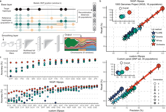
Orchestra is a LAI algorithm that consists of a two-stage pipeline: an original deterministic base layer and a smoothing module based on a deep learning architecture that combines elements of convolutional neural networks47 and attention-based (transformer) mechanisms48. Orchestra’s base layer is a deterministic algorithm modeled on recombination, built on the assumption that shared homologous haplotypes are identical by descent (IBD). We expect that a person would share longer DNA segments with individuals from the same population and shorter segments with individuals from remote populations. The base layer looks at each window on a chromatid and finds the minimum number of segments that would be needed to reconstruct that window when those segments are sampled from specific, carefully selected reference populations. We refer to this value as recombination distance. In this study, each chromosome was divided into windows spanning 600 SNPs.
The base layer works as a greedy search algorithm. In each window, the algorithm starts at the first position, looking for the longest continuous matching haplotype in a reference population. Where the match stops, the algorithm starts again from that position to find the longest local match, and so on. This is carried out using a NumPy array of the (boolean) matches at any given position between the sample and the reference sequences (as rows) and using the product along the rows. This allows to accelerate the computation in a trade-off of some use of memory for extra speed, plus it allows the calculation to be parallelized easily across the data. The procedure is repeated until it produces a vector of recombination distances against all reference populations.
The smoothing layer uses the vector of recombination distances produced by the base layer as an ancestry fingerprint that gets converted to a measure of ancestry in terms of probabilities. This layer is designed to give higher weights to low-frequency classes (populations) in the loss function to handle class imbalance effectively. Then, the information from surrounding and more remote windows is factored in, to output a final ancestry label. To do this effectively, the smoothing layer consists of two different types of layers: convolutional and attention-based. There are five convolutional and two attention layers. The attention layers are sandwiched between the third and fourth, and the fourth and fifth convolutional layers. The convolutional layers are moving filters that generate different insights from the base layer output and retain the information in parallel. Whereas in a normal convolutional neural network we would have pooling layers in between the convolutional layers47, we use attention layers that process the result of the parallel filters as a (similarity) vector space that would typically be the output of an embedding into an n-dimensional vector space in a transformer architecture48 to provide global information flow using proximity in this convolutional vector space. The purpose of the convolutional layers is to process information at the window level in the case of the first two convolutional layers and to bring local information concerning other nearby windows in the case of the third, fourth and fifth convolutional layers. The closest windows tend to have a larger impact due to the fact that windows tend to form blocks of a given ancestry, but the attention mechanism allows the use of a comprehensive context to weight the base layer outputs from all other windows. In this regard, the attention augments the local convolutional layers with global information flow. The simplification of the attention layer relative to regular transformer architecture allows the use of a context long enough to span the entirety of the windowed data for a chromosome pack. The final convolutional layer provides the output in terms of probabilities. The population that is assigned the maximum probability is given as the final ancestry.
Due to computation limitation, the smoothing layer was not trained on all chromosomes at a time, but was instead trained on chromosome packs (1/2, 3/4,…, 17/18, 19/20/21/22). Training on a larger set of chromosomes at a time, or even the entirety of the genome, is expected to further increase the accuracy of the smoothing layer.
During the training phase, where Orchestra adjusts its smoothing layer parameters (weights and bias terms) using simulated admixed individuals, it is inevitable that subsequent generations will include direct descendants of the original samples (see ‘Simulated Admixed Individuals’). This means the same haplotypes are present in both the reference and target sets, potentially leading to an overfitted model. To minimize bias from using source samples of the synthetic admixed data as reference sequences for population classification, Orchestra’s base layer algorithm was modified to remove the best matching haplotypes from the entire training set using a greedy matching algorithm, under the assumption that these best matches represent the ‘ancestral’ samples of the simulated genomes. Once the model is trained, it can be applied to any separate testing cohort.
Reference panel
Despite the increasing number of publicly available datasets, obtaining a comprehensive and balanced reference panel remains a challenging step in ancestry deconvolution. Here, we used 1KGP-16pops (N = 1365), composed of unrelated non-admixed individuals collected by 1KGP, as the gold standard dataset, which enables easy accuracy comparisons with previously published studies. Next we created the custom-35pops dataset (N = 10,169), where we aimed to assemble a genome-wide dataset of non-admixed modern samples from diverse populations around the globe49,50,51,52,53,54,55,56,57,58,59,60,61,62,63,64,65,66,67,68,69,70,71,72,73,74,75,76,77,78,79,80,81,82,83. A detailed list of all data mined for this study can be found in the Supplementary Table 1. The granularity we were able to achieve on each continent was largely dependent on the number and diversity of samples we had available. Where samples were limited or not divergent enough based on initial experiments, we grouped populations into meaningful, broader geographic regions with shared genetic ancestry. Precise information about dataset preparation and merging can be found in Supplementary Methods.
Our custom-35pops dataset is composed of many studies, including genotyping arrays and WGS, which gave rise to artifacts that interfered with the detection of biological patterns due to batch effects84. As to our knowledge, there are no effective and systematic algorithms to remove them, therefore we applied conventionally recommended quality control measures85 (see Supplementary Methods).
After batch effect removal, we used two complementary strategies to identify admixed individuals. The first was PCA-UMAP, an existing protocol for dimensionality reduction86 that allowed us to visualize relatedness among individuals. The second was GNN-tSNE, where we used tsinfer5 to infer the tree sequences for our dataset and compute the genealogical nearest neighbors (GNN), to which we applied t-distributed stochastic neighbor embedding (t-SNE), another non-linear dimensionality reduction technique. Outliers (i.e., admixed genomes) were removed automatically using a K-Nearest Neighbor (KNN) algorithm (see Supplementary Methods).
To detect Native American ancestry in target genomes, we generate a reference panel of 100 pure in silico Native American genomes (see Supplementary Methods).
Simulated admixed individuals
SLiM v3.723 was used to generate admixed genomes based on single-ancestry populations from the reference panel. We forward simulated 1–6 generations of admixture. True local ancestry of every position in every simulated individual was tracked across generations using the tree-sequence recording function, and browsed with tskit and pyslim packages87. HapMap recombination map was supplied for modeling the non-uniform recombination events across the genome.
Given that SLiM does not support simulations with more than one chromosome, we ran each chromosome independently but followed the same mating scheme over generations to obtain whole-genome simulations with the same ancestors for all chromosomes. We tracked the pedigree obtained in the first chromosome run by tagging each simulated individual and each pair’s offspring, and reproduced the same genealogy for the others.
We simulated a fully intermixed scenario where all individuals from populations in the reference panel had an equal probability of contributing to mating, with no specific rates assigned to population mixing, as individuals were chosen entirely at random for each generation. By generation 6, each haploid genome could contain ancestry from up to 32 populations. The expected median number of admixed populations per haploid genome is ~1, 2, 4, 7, 13, and 21 for generations 1 through 6. We also implemented a more realistic non-random model where individuals preferentially mate within their continent (e.g., Europeans, Western Asians, and North Africans; Sub-Saharan Africans; Central and South Asians; and East and Southeast Asians), with a 10% migration rate per generation. We found that the benchmarking results were nearly identical. Thus, we opted to train Orchestra in the fully intermixed random-mating scenario to ensure robustness.
We ran a non-Wright-Fisher model of evolution, since we implemented a couple of modifications. Despite choosing parents via random sampling, we avoided inbreeding by recording pedigree information and thus identifying the degree of relatedness of each pair selected. Only individuals that were not close relatives were allowed to mate (at least a coefficient of relationship
Benchmarking
For benchmarking, we inferred local ancestry with RFMix v2.039, FLARE v0.1.010 and Gnomix11. We split the samples randomly into training (80%) and testing (20%) cohorts, and measured performance globally, per generation, and per population. We report precision and recall as accuracy measures with scikit-learn88, which are computed per population; i.e., the number of true positives (TP), true negatives (TN), false positives (FP), and false negatives (FN) is calculated with respect to the selected population as the positive class. In the case of TN and FN, the prediction can be anything other than the population under consideration. We additionally report a commonly used alternative measure for accuracy by assessing each method with Pearson’s r2. We calculated the coefficient of determination by comparing both the inferred and the true local ancestry label per haplotype, as well as the diploid ancestry dose by counting the number of ancestry labels (0, 1 or 2) per site. Values of r2 were estimated for each ancestry separately and the weighted mean r2 across all ancestries was reported per generation.
All programs were supplied with the same training (as reference panel) and test (as target) genotype data, and the HapMap recombination map. Statistical parameters were kept at default values with the following exceptions: the Gnomix model was trained from scratch and its accuracy was optimized in our scenario using Large mode, smooth_size: 100, context_ratio: 0.10 and window_size_cM: 0.5; whereas the number of generations for RFmix was specified with -G 6. For the 1KGP-16pops WGS panel, we processed variants using a MAF filter (
We assembled a new panel using UKBB samples for additional benchmarking, providing a distinct and independent validation dataset to assess Orchestra’s ability to generalize beyond the original test set. We picked samples that (1) closely aligned with their respective ancestral groups based on both PCA + UMAP and GNN+t-sne dimensionality reduction approaches but were not incorporated into the final reference panel due to sample size limits, and/or (2) they were close to their population cluster but overlapped with other/s and therefore were excluded at the quality control stage. For regions like the Republic of Ireland, Wales, Scotland, and England, which had a larger sample base in this panel, we considered a maximum of 1000 samples per region. Altogether, we collected 10,241 samples spanning 103 countries. Accuracy was evaluated by attributing the appropriate ancestry label from our ancestry reference panel to each country and then comparing it with the LAI results from each method (Supplementary Fig. 2c).
Retracing genetic histories
We simulated Latin American individuals from Southern (SPP and ITA) and Northern (FRG and BRI) Europeans, Western (GSE, GLS and NGE) and Central and Southern (SAF) Africans and artificially-reconstructed Native Americans (NAM) from our custom ancestry panel. Simulations were performed by emulating genetic intermixing for 12 generations using SLiM23. Details about the simulations can be found in the Supplementary Methods section. For our benchmarking evaluation, we partitioned the samples randomly into training and testing groups, allocating 80% and 20% of the simulations, respectively, to assess Orchestra against other LAI tools. We ensured that training and testing samples never coincided across the three simulated regional datasets, guaranteeing consistent comparison metrics. We evaluated the performance in terms of precision and recall for each Latin American region using scikit-learn.
For real-world data analysis, we identified UKBB participants born in the Americas using birthplace codes (data-field f.20115), specifically from South America ( >C.600) and North America (C.400-C.500). Additionally, we incorporated admixed American 1KGP samples (codes: MXL, PUR, CLM and PEL). We then extracted the composite SNP set from both the imputed UKBB and whole-genome 1KGP sets and ran Orchestra for LAI assessment. Samples with ancestry patterns closely matching British ancestry (BRI + FRG + SCA > 80%) were discarded (Supplementary Fig. 23).
Finally, we applied Orchestra to all UKBB samples not selected for our reference panel, and samples obtained from various datasets, especially from Reich lab, that were not included in our reference panel because they belonged to ethnic groups other than those found in our 35 reference populations (Supplementary Figs. 5–7).
Ancestral mapping
We created 35 different reference panels for each target population, by excluding the target population from its own reference panel. Orchestra was then trained on each reference panel and applied to the target population. Due to computational limitations, training on these 35 datasets was limited to chromosomes 17–22. The admixture proportions obtained for each population were converted into a matrix of distances that were projected onto two-dimensional space using the SMACOF (Scaling by MAjorizing a COmplicated Function) algorithm implementation of scikit-learn using the sklearn.manifold.MDS function with the option metric=True to convert a non-Euclidean symmetric dissimilarity matrix to coordinates in 2 dimensional space. The SMACOF algorithm uses a random initialization followed by stress majorization to iteratively minimize a stress function given by the squared difference between the dissimilarity matrix entries and the Euclidean distances between the points in 2 dimensional space. To create the matrix of distances, the obtained series of ancestry proportions were first averaged over the samples for each population. These averages were then assembled inside a two dimensional matrix with each dimension being the number of the populations, with 0 on the diagonal. 0.00000000000000001 was then added to all the entries of the matrix to remove any 0 entries and allow the reciprocal to be taken. The matrix was then added to its transpose, to make it symmetric, which was a necessity to apply the algorithm. The reciprocal was taken to convert the similarity measures of proportions into dissimilarity, before being input into the sklearn.manifold.MDS function to produce the coordinates.
Detecting natural selection signatures
To detect natural selection in admixed populations we focused on the Fadm and LAD statistics described in Cuadros–Espinoza et al.34. We explain the steps in detail in the Supplementary Methods section. We first scanned the genomes of seven admixed populations already analyzed in Cuadros–Espinoza et al.34, leveraging either publicly available genotypes89,90,91,92,93 or an appropriate proxy from the UKBB or Reich lab. These served as positive controls to gauge the accuracy in replicating previously identified signals. Detailed information on the datasets and the respective references for these populations is provided in Supplementary Fig. 15. External datasets were lifted over to hg38 and imputed, followed by the extraction of the composite SNP set for LAI assessment with Orchestra. In the absence of a direct proxy for Malagasy, we considered African, Black or mixed participants from the UKBB with a significant proportion of Austronesian (SEA + FIL > 1%) and South African (SCA > 20%) ancestry and low Indian (PNI + BEI + SSI
We then extended this methodology to the White British from the UK, where we treated the British population as admixed, and looked at the Scandinavian component in British genomes. We analyzed 415,859 British participants from the UKBB dataset with detailed birth location information within the UK (using north and east coordinates or data-fields f.129 and f.130). Birth locations were categorized according to the 2018 NUTS Level 2 boundaries (counties) from the Office for National Statistics (https://data.gov.uk/). Shapefiles were loaded and processed using rgdal R package. Scandinavian (SCA) average percentage was next computed based on individuals mapped to each specific geographic area in Britain. Additionally, we retrieved the index of place names in Great Britain (July 2016) to pinpoint those towns or cities with Viking-origin names, suggesting past Viking settlements (evidenced by suffixes such as -by, -thorpe, or -toft). Next we took 287,346 British samples that showed traces of SCA ancestry. Due to the emergence of a signal in chromosome 10, we wanted to ensure the validity of this observation by analyzing three additional sets of British samples, each varying in their Scandinavian ancestry enrichment. Specifically, we assessed British samples bearing >1%, >5%, and >20% Scandinavian ancestry (Supplementary Fig. 16). Given that SCA is the population with the lowest accuracy in our panel (Fig. 1c), we removed 10 windows from the telomeric regions. We further refined the signal by adjusting the averaged SCA ancestry percentage present in every window against the standard deviation observed in its chromosome pack. Chr10 signal remained consistent across sets as illustrated in Supplementary Fig. 16.
OpenTargets
We selected variants that surpassed the established P value significance threshold and explored the Open Targets database (https://www.opentargets.org/) for potential target genes. These genes were then ranked based on the aggregate score obtained from all variants.
GWAS enrichment
To investigate if the number of GWAS Catalog (http://www.ebi.ac.uk/gwas/) [release 2023-07-20] hits in the selected region is higher than expected by chance, we crossed GWAS Catalog signals (P -8) with 1000 Genomes Project variants and grouped together those in high LD (r² ≥ 0.8) and associated to the same phenotype. Enrichment P values were calculated by comparison with a null distribution from random genomic regions as a background model, controlling by region size and excluding gaps, sexual chromosomes and the major histocompatibility complex region, known to harbor a vast number of associations. Since the size of the region to be studied is ~2.5 Mb, the number of simulations cannot be too large without covering the entire genome and having overlapping simulations. Thus, we also tested GWAS enrichment with a Fisher’s exact test, which showed very similar results (odds ratio correlation: R² = 0.97; P value correlation: R² = 0.69). We selected this latter statistic for the analyzes due to its higher statistical power. GWAS Catalog reported traits were grouped by parent categories according to EFO terms from the ontologyIndex R package. P values were adjusted by Bonferroni correction.
To determine whether this region in chr10 of Scandinavian ancestry, as opposed to British, would result in an increase or decrease for each GWAS phenotype, we computed the frequency difference of the GWAS variants between these two populations using our custom ancestry panel, providing insight into the potential direction of the effect resulting from this shift in ancestry.
Phenotype mapping
Following the association strategy of admixture mapping, we contrasted the proportion of SCA ancestry among cases and controls to evaluate the influence of the chr10 locus on phenotypes gathered by the UKBB. For that, we took main and secondary ICD10 codes and self-reported illness codes (data-fields f.41202, f.41204 and f.20002, respectively). Phenotypes represented by fewer than 100 cases were excluded. Given the absence of significant phenotypes using the Fisher exact test and subsequent P value correction, we filtered phenotypes based on their nominal P value (P
Reporting summary
Further information on research design is available in the Nature Portfolio Reporting Summary linked to this article.