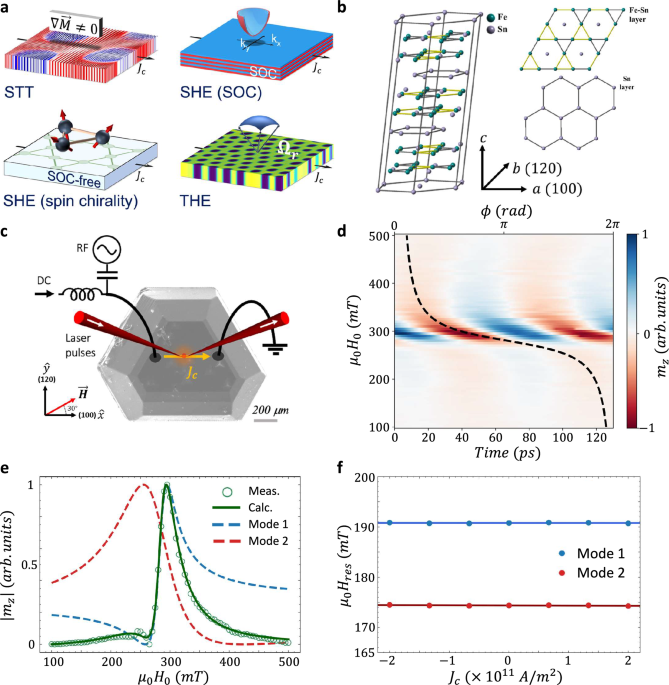
The Fe3Sn2 crystal has a rhombohedral unit cell which belongs to the \({{\rm{R}}}\bar{3}{{\rm{m}}}\) space group. It consists of alternating double kagome Fe-Sn and hexagonal Sn layers stacked along the c-axis (Fig. 1b) having lattice constants of \(a=b=5.338\,{{\text{\AA }}}\) and \(c=19.789\,{{\text{\AA }}}\) in hexagonal coordinate system34. The adjacent kagome Fe-Sn layers are offset, and each consists of two different Fe-Fe bond lengths of \(2.732\,{{\text{\AA }}}\) and \(2.582\,{{\text{\AA }}}\). Crystals of Fe3Sn2 were synthesized by chemical vapor transport reaction as described in ‘Methods’. Figure 1c presents a scanning electron microscope (SEM) image of the crystal.
The magnetization dynamics were studied using an optically probed STFMR technique (OSTFMR)33,35,36. An RF charge current of frequency \(f\) was passed through the crystal and excited the dynamics. The responses were probed using a femtosecond laser that was phase-locked to the RF signal. The OOP component of the RF magnetization, \({m}_{z}\), was probed using the magneto-optical Kerr effect (MOKE) and an optical delay line provided the temporal resolution. The current was passed along the \(\hat{x}\) direction corresponding to the [100] crystal axis and the external magnet field \(\vec{H}\) of magnitude \({H}_{0}\) was applied in the sample plane at \({\theta }_{H}=30^\circ\) with respect to the [100] axis as indicated in Fig. 1c (see ‘Methods’ for further details).
An example of an OSTFMR trace at \(14\,{GHz}\) is presented in Fig. 1d. The trace presents \({m}_{z}\left(t\right)\) as a function of \({H}_{0}\) in which a resonance peak appears at \(\sim \,300\,{mT}\). The extracted phase response, \(\phi \left({H}_{0}\right)\), is represented by the black dashed line. Interestingly, \(\phi \left({H}_{0}\right)\) reveals a total phase shift, \(\Delta \phi\), of \(\sim \,2\pi\) accumulated across the resonance rather than the expected \(\pi\) shift, indicating that actually two resonance modes were measured. This is confirmed by plotting the amplitude response \(\left|{m}_{z}\left({H}_{0}\right)\right|\) presented in Fig. 1e that reveals a secondary feature at \(\sim \,250\,{mT}\). Namely, the AC magnetic susceptibility consists of two Lorentzian lines \({\chi }_{m}={\sum }_{i={\mathrm{1,2}}}{A}_{i}\cdot \frac{1}{\left({H}_{{re}{s}_{i}}^{2}-{H}_{0}^{2}\right)+i{H}_{0}\Delta {H}_{i}}\cdot {{{\rm{e}}}}^{i{\phi }_{i}}\) where \({A}_{i}\), \({H}_{{re}{s}_{i}}\), and \(\Delta {H}_{i}\) are the amplitude, resonance field, and linewidth of each resonance mode, and \({\phi }_{i}\) is the phase relative to the RF excitation. The reconstructed \({m}_{z}\left({H}_{0}\right)\) is presented as well in Fig. 1e together with the two retrieved modes and agrees well with the measurement. Using micromagnetic simulations that account for the exchange, dipole-dipole, tilted UMA, and Zeeman energies (see ‘Methods’), we find that the lower (higher) resonance field corresponds to the CCW (breathing) mode. In the general case, the CW mode should also be excited, however, it is typically of a smaller amplitude while the combined effect of frustration and strong exchange interaction further suppress its excitation1. The driving RF torque can stem from the RF Oersted or RF spin-torque. In frustrated magnets, an IP RF Oersted field can only drive the CCW mode1,27. In contrast, the RF spin-torque consists of IP and OOP components that can excite also the translational mode. Namely, the excitation of the two orthogonal modes implies the generation of RF spin-torque in the crystal. The negligible self-induced Oersted torque33 was verified by passing a DC current density \({\vec{J}}_{c}\) of magnitude \({J}_{c}\) which had no effect on \({H}_{{re}{s}_{i}}\) as seen in Fig. 1f.
The same analysis was repeated for additional frequencies. The top panels of Fig. 2a show characteristic spectra measured at \(6\), \(8\), \(12\), and \(14\,{GHz}\). At high frequencies, distinct resonances appear whereas at low frequencies the spectrum is random. This behavior is summarized by plotting the \(f-{H}_{{re}{s}_{i}}\) dispersion relations presented in the main panel of the figure. A phase transition is seen at \(\sim \,10\,{GHz}\) (\(\sim 175\,{mT}\)). This transition can be understood from the dynamical micromagnetic simulations. To this end, the static textures were first determined and are presented in the top panels of Fig. 2b. A disordered phase is seen at \({H}_{0}=0\) that evolves into a stripe phase at \(75\,{mT}\) after which an ordered lattice phase emerges. When \({H}_{0}\) is further increased, the texture gradually saturates. The dynamical responses were obtained from the Fourier transform of the impulse response of the mean OOP magnetization \({M}_{z}\) and are presented in the main panel of Fig. 2b. The calculated dynamics correlate with the magnetic phase transitions and reproduce the trends seen in the measurements: scattered resonance peaks measured at \({\mu }_{0}{H}_{0} \, and a homogeneous monotonic dispersion curve consisting of two modes at high \({H}_{0}\). Indications of the stripe phase are also found in the measurement as seen in the spectrum of \(8\,{GHz}\) which is significantly broader due to the higher motional degrees of freedom. From the calculations, \(Q=0\) was determined in the lattice phase (see Supplementary Note 3). Following the conventional terminology, we use the term skyrmion resonance although the magnetic texture is topologically trivial.
Fig. 2: Measured and calculated resonance dynamics of Fe3Sn2.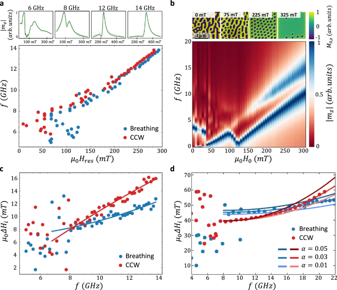
a Measured dynamical response. Top panels present measured \(\left|{m}_{z}\right|\) as a function of \({H}_{0}\) at \(6\), \(8\), \(12\), and \(14\) \({GHz}\) (light green open circles). Reconstructed responses are indicated in green solid line. Data is presented in normalized units. Main panel: Frequency dispersion relations of the breathing and CCW resonance modes. b Micromagnetic dynamical simulations. Top panels present the calculated textures at \({{\mu }_{0}H}_{0}=0\), \(75\), \(225\), and \(325\,{mT}\). The textures are represented by plotting the equilibrium OOP component of the magnetization, \({M}_{0,z}\). The main panel presents the calculated frequency response of \(\left|{m}_{z}\right|\) as a function of \({H}_{0}\) for \(\alpha=0.05\). Each response was normalized to its peak value. c Measured resonance linewidths (\(\Delta {H}_{i}\)) of CCW and breathing modes as a function of \(f\). Solid lines represent a fit to a second order polynomial function. d Calculated \(\Delta {H}_{i}\) of the two modes. Solid lines illustrate the calculation for \(\alpha=0.01\), \(0.03\), and \(0.05\). In (a, c, d) data of the breathing and CCW modes are indicated by blue and red colors, respectively.
Interestingly, features appearing in the measured resonance linewidths are also reproduced in the calculation. Figure 2c presents the measured \(\Delta {H}_{i}\) as a function of \(f\). It is seen that \(\Delta H\) of the CCW mode increases more rapidly with \(f\) as compared to the breathing mode. The same behavior is seen in the calculated \(\Delta {H}_{i}\) presented in Fig. 2d which was obtained using \(\Delta {H}_{i}={\left(\frac{\partial {f}_{{res}}}{\partial {H}_{0}}\right)}^{-1}\Delta {f}_{i}\). The overall broader calculated \(\Delta {H}_{i}\) stems from the inhomogeneous broadening induced by the interfaces of the finite calculation space. A Gilbert damping of \(\alpha=0.032\pm 0.008\) was evaluated from the \(f\) dependent \(\Delta H\) broadening of the CCW mode in the range \(f \, > \, 10 \,{GHz}\) which is comparable to previously measured values in thin films of Fe3Sn237. In the CCW mode, the spins undergo a local precessional trajectory about an effective field. Therefore, the Rayleigh viscous-like damping process manifests in the measured quasi-linear dependence at high \(f\). In contrast, in the breathing mode, the spins follow a non-conical expansion and contraction-type motion that results in a weaker dependence of \(\Delta H\) on \(f\).
Next, we examine the influence of \({J}_{c}\) on the skyrmion resonance linewidth. In the following experiments, the current was passed along the [100] axis. Figure 3a–c present the measured data for the disordered, stripe, and lattice phases by plotting the variation of \(\Delta {H}_{i}\) relative to the zero-bias linewidth \(\Delta {H}_{i}^{0}\). In the disordered phase, a significant random modulation of \(\Delta {H}_{1,2}\) appears which stems from switching of the textures by \({J}_{c}\)7\(.\) In the stripe and lattice phases, \(\Delta {H}_{1}\) increases monotonically with \({J}_{c}\) while \(\Delta {H}_{2}\) decreases. In FMR measurements of a non-textured saturated magnetization, the linewidth is directly related to the magnetic losses, therefore, a current induced linewidth broadening is indicative of a damping-like torque. However, in textured magnets, the relation between the Slonczewski damping-like torque and resonance linewidth is not straight forward due to the anisotropic nature of the torque. To elucidate this behavior, the torque was included in the micromagnetic simulations by introducing STT and SOT terms of the forms \({\tau }_{{STT}}\widehat{{{\boldsymbol{m}}}} {{{\times }}}\widehat{{{\boldsymbol{m}}}} {{{\times }}}({\vec{{{\boldsymbol{J}}}}}_{{{\boldsymbol{c}}}}\nabla )\widehat{{{\boldsymbol{m}}}}\) and \({\tau }_{{SOT}}{J}_{c}\widehat{{{\boldsymbol{m}}}}\times \widehat{{{\boldsymbol{m}}}}\times \widehat{{{\boldsymbol{s}}}}\), respectively. Here, \({\tau }_{{STT}}\) and \({\tau }_{{SOT}}\) are coefficients of the two torques and \(\hat{s}\) is the spin polarization of the SOT (see ‘Methods’). Figure 3d–f present the simulation results for the case of a DC STT by plotting the \({J}_{c}\)-dependent \(\Delta {H}_{i}\). In the disordered phase, a \({J}_{c}\)-induced texture switching takes place which manifests in the random modulation of \(\Delta {H}_{i}\). However, no discernable modulation of the linewidth is observed in the stripe and lattice phases. This trend persists up to a critical value of \({J}_{c}\) after which the texture switches also in these phases (see Supplementary Note 4). In contrast, the application of a DC SOT leads to the modulation of \(\Delta {H}_{i}\) observed experimentally. The SOT case was studied for \(\hat{s}\) along the three principal axes as presented in Fig. 3g–i. In the disordered phase, the texture switching is reproduced while a monotonic dependence of \(\Delta {H}_{i}\) on \({J}_{c}\) is calculated in the stripe and lattice phases. It is seen that the case of \(\hat{{{\boldsymbol{s}}}}=-\hat{{{\boldsymbol{z}}}}\) best reproduces the measurements. Alternatively, also a combination of \(\hat{{{\boldsymbol{s}}}}=-\hat{{{\boldsymbol{z}}}}\) and \(\hat{{{\boldsymbol{s}}}}=-\hat{{{\boldsymbol{x}}}}\) may result in a similar trend. In the stripe phase, the inhomogeneous broadening is more significant. Therefore, the effective spin Hall angle was estimated from the CCW mode at the lattice phase for \(\hat{{{\boldsymbol{s}}}}=-\hat{{{\boldsymbol{z}}}}\) which resulted in \({\theta }_{{SH}}^{{eff}}=0.027\pm 0.006\) (see ‘Methods’).
Fig. 3: Measured and calculated current induced skyrmion resonance linewidth broadening at the disordered, stripe, and bubble lattice phases.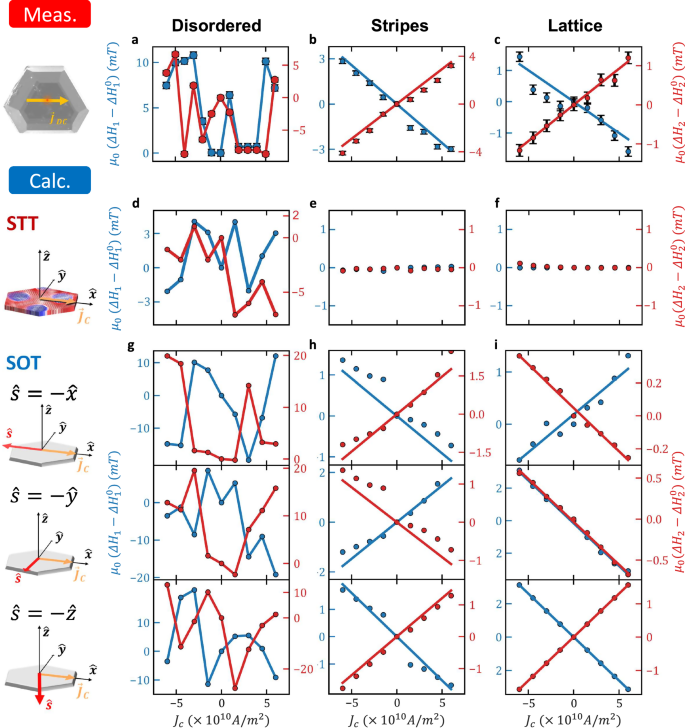
a–c Measured \(\Delta {H}_{i}-\Delta {H}_{i}^{0}\) at \(5\), \(10\), and \(12\) \({GHz}\). d–f Calculated \(\Delta {H}_{i}-\Delta {H}_{i}^{0}\) for DC STT. g–i Calculated \(\Delta {H}_{i}-\Delta {H}_{i}^{0}\) for DC SOT. The figures present the calculation for \(\hat{{{\boldsymbol{s}}}}=-\hat{{{\boldsymbol{x}}}}\),\(\,\hat{{{\boldsymbol{s}}}}=-\hat{{{\boldsymbol{y}}}}\), and \(\hat{{{\boldsymbol{s}}}}=-\hat{{{\boldsymbol{z}}}}\). In the simulations, \(\Delta {H}_{i}\) for the disordered, stripe, and lattice phases were calculated at \({\mu }_{0}{H}_{0}=10\), \(100\), and \(250\,{mT}\), respectively, corresponding to the measurements at \(5\), \(10\), and \(12\) \({GHz}\). Left, middle, and right columns correspond to the disordered, stripe, and bubble lattice phase, respectively. Red and blue solid lines correspond to the CCW and breathing modes, respectively.
The THE is a useful probe of texture-driven transport phenomena and appears as an anomaly in the AHE response38,39. Figure 4a presents temperature dependent Hall resistivity \({\rho }_{{xy}}^{\perp }\) which consists of the contributions of the ordinary Hall effect (OHE), AHE, and THE40. For high \(\left|{H}_{0}\right|\), \({M}_{z}\) is saturated so that the THE vanishes and the AHE dominates. At lower \(|{H}_{0}|\), the THE arises. This is readily seen in Fig. 4b by plotting the THE contribution, \({\rho }_{{xy}}^{{THE}}\), obtained by subtracting the contributions of the OHE and AHE (see ‘Methods’). \({\rho }_{{xy}}^{{THE}}\) survives up to \(700\,{mT}\) where the maximal value occurs at \({{\mu }_{0}H}_{0}\approx 300\,{mT}\) and accounts for nearly 50% of \({\rho }_{{xy}}^{\perp }\). This highlights the significant role of the real-space Berry curvature in Fe3Sn29. Lorentz transmission electron microscopy (LTEM) images presented in Fig. 4c further support this conclusion revealing that a skyrmion lattice forms having \(Q\, \ne \, 0\) at the maximal value of \({\rho }_{{xy}}^{{THE}}\).
Fig. 4: Angle and temperature dependent DC Transport measurements.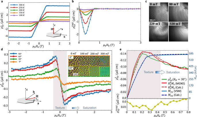
a Temperature dependence of \({\rho }_{{xy}}^{\perp }\) with OOP \(\vec{{{\boldsymbol{H}}}}\). b Temperature dependence of \({\rho }_{{xy}}^{{THE}}\). \({\rho }_{{xy}}^{{THE}}\) is extracted by subtracting the OHE and AHE contributions from \({\rho }_{{xy}}^{\perp }\). c LTEM images at \(300\,{K}\) for \({\mu }_{0}{H}_{0}=0\), \(80\),\(\,220\), and \(320\,{mT}\) in the OOP configuration. d PHE measurements of \({\rho }_{{xy}}^{\parallel }\) for IP \(\vec{{{\boldsymbol{H}}}}\) applied at \({\theta }_{H}=\) \({0}^{\circ }\), \(3{0}^{\circ }\),\(\,6{0}^{\circ }\), and \(9{0}^{\circ }\) with respect to the \([100]\) axis. Inset presents calculated magnetic textures for \({\theta }_{H}={0}^{\circ }\) and \(3{0}^{\circ }\). e Extraction of the topological contribution, \({\rho }_{{xy}}^{{TPHE}}\), at \({\theta }_{H}=3{0}^{\circ }\). Upper panel: Measurement of \({\rho }_{{xy}}^{\parallel }\) (green solid line) together with the measured \({R}_{s}^{\parallel }{\mu }_{0}{M}_{z}\) (red line) at \({\theta }_{H}={30}^{\circ }\). \({M}_{z}\) was measured using a MOKE setup at \({\theta }_{H}={30}^{\circ }\) (red line). \({R}_{s}^{\parallel }\) was determined from \({\rho }_{{xy}}^{\parallel }\) at the saturated magnetization regime. Saturation conditions were verified by calculating \({M}_{z}\) at \({\theta }_{H}={30}^{\circ }\) (red dashed line) and by measuring \({M}_{{xy}}\) using a VSM (blue solid line). Calculated \({M}_{{xy}}\) (blue dashed line) reproduces the measured \({M}_{{xy}}\) in saturation. Lower panel presents the extracted \({\rho }_{{xy}}^{{TPHE}}\).
In contrast to the measurement of the THE, in the OSTFMR measurements \(\vec{H}\) was applied in the sample plane. Therefore, the planar Hall resistivity \({\rho }_{{xy}}^{\parallel }\) was also measured and is presented in Fig. 4d. In this geometry, the tilted UMA produces a non-vanishing \({M}_{z}\) giving rise to the usual AHE that originates in the \(k\)-space band topology in addition to the effective magnetic field that emerges from the localized spin structure in real-space. We refer to these contributions as the \(k\)-PHE and topological PHE (TPHE) analogously to the AHE and THE terms of \({\rho }_{{xy}}^{\perp }\). Accordingly, \({\rho }_{{xy}}^{\parallel }={R}_{s}^{\parallel }{{\mu }_{0}M}_{z}+{P}_{z}^{\parallel }({H}_{0}){R}_{0}^{\parallel }{b}^{z}\) where \({R}_{s}^{\parallel }\) and \({R}_{0}^{\parallel }\) are the \(k\)-PHE and TPHE coefficients, respectively, \({P}_{z}^{\parallel }\left({H}_{0}\right)\) is the net \(\hat{z}\) spin polarization of the charge carriers, and \({b}^{z}\) is the fictitious gauge field emerging from the real-space Berry curvature. \({P}_{z}^{{||}}\left({H}_{0}\right)={C}_{0}\cdot |{M}_{z}/{M}_{s}|\) with the constant C0 determined by the material band structure and \({M}_{s}\) is the saturation magnetization. The figure presents \({\rho }_{{xy}}^{\parallel }\) for different IP \({\theta }_{H}\) angles together with the calculated magnetic textures at \({\theta }_{H}={0}^{\circ }\) and \(3{0}^{\circ }\) (textures for \({\theta }_{H}=6{0}^{\circ },\,9{0}^{\circ }\) are presented in Supplementary Note 5). \({\rho }_{{xy}}^{\parallel }\) is substantially smaller than \({\rho }_{{xy}}^{\perp }\) due to the smaller \({M}_{z}\) and \({P}_{z}^{\parallel }\) in the planar geometry. The non-monotonic behavior of \({\rho }_{{xy}}^{\parallel }\) is a hallmark of the formation of a multi-domain texture in PHE measurements41. For \({\theta }_{H}={30}^{\circ }\) at which the OSTFMR measurements were carried out, the maximal value of \({\rho }_{{xy}}^{\parallel }\) occurs at \(198\,{mT}\) corresponding to the bubble lattice phase. At \({\theta }_{H}={0}^{\circ }\), the simulations reveal that the lattice phase does not form, therefore, \({\rho }_{{xy}}^{\parallel }\) should not exhibit a peak. Indeed, the measured \({\rho }_{{xy}}^{\parallel }\) is smaller as compared to the case of \({\theta }_{H}={30}^{\circ }\), however, a slight peak is still observed and stems from a slight misalignment of \(\vec{H}\) as verified in Supplementary Note 6. At \({\theta }_{H}={30}^{\circ }\) and \({|{\mu }_{0}H}_{0}| > 400\,{mT}\), the texture saturates resulting in \({b}^{z}\approx 0\) and the response purely stems from the \(k\)-space PHE. In the presence of the tilted UMA axis, \({M}_{z}\) saturates to different values depending on \({\theta }_{H}\). Consequently, \({\rho }_{{xy}}^{\parallel }\) approaches a different limit as \({\theta }_{H}\) is varied. The different saturation limits were also verified in the calculation (see Supplementary Note 6).
To determine the TPHE contribution at \({\theta }_{H}={30}^{\circ }\), \({M}_{z}\) was measured using a static MOKE. This data is presented in Fig. 4e (red solid line) together with the measured \({\rho }_{{xy}}^{\parallel }\left({\theta }_{H}={30}^{\circ }\right)\) (green solid line). \({M}_{z}\) is represented by plotting \({R}_{s}^{\parallel }{\mu }_{0}{M}_{z}\) where \({R}_{s}^{\parallel }\) was determined from the saturated \({\rho }_{{xy}}^{\parallel }\) responses at high \({H}_{0}\). The TPHE contribution \({\rho }_{{xy}}^{{TPHE}}\) was extracted by subtracting \({R}_{s}^{\parallel }{{\mu }_{0}M}_{z}\) from \({\rho }_{{xy}}^{\parallel }\) and is plotted in the lower panel of the figure. This procedure was additionally validated by vibrating sample magnetometer (VSM) measurements of the IP magnetization, \({M}_{{xy}}\) (blue solid line), and a numerical calculation of \({M}_{z}\) and \({M}_{{xy}}\) (red and blue dashed lines, respectively) which reproduced the measurement in the saturation regime. It is seen that \({\rho }_{{xy}}^{\parallel }\) primarily stems from the \(k\)-space PHE while the maximal contribution of \({\rho }_{{xy}}^{{TPHE}}\) is \(\sim 10.7\,\%\) obtained at \(\sim 320\,{mT}\) and is significantly smaller than the relative contribution of the THE in the measurement of \({\rho }_{{xy}}^{\perp }\). Once more, the maximal value of \({\rho }_{{xy}}^{{TPHE}}\) corresponds to a lattice phase as seen from the calculated textures displayed in Fig. 4d. At \(250\,{mT}\) where \({\theta }_{{SH}}^{{eff}}\) was extracted, \({\rho }_{{xy}}^{{TPHE}}\) accounts for \(8.5\,\%\) of \({\rho }_{{xy}}^{\parallel }\).