Data collection and cleaningFall armyworm occurrence records
FAW occurrence records were obtained from the following sources: the Global Biodiversity Information Facility58 (GBIF), Butterflies and Moths of North America59 (BAMONA), the European and Mediterranean Plant Protection Organization12 (EPPO), and the Center for Agriculture and Biosciences International60 (CABI), as well as published datasets44,52 and occurrence records in the literature. For the occurrence records in the literature, we used the keywords “Spodoptera frugiperda [country name]” in Google Scholar for each country where FAW’s presence is confirmed by EPPO (last update for all sources: February 2024). All records reported in GBIF were acquired using the “rgbif”61 R package (R software version 4.3.362) and selecting the corresponding GBIF taxon ID (5109855) for Spodoptera frugiperda.
We conducted a data cleaning process for the GBIF occurrence dataset by using the “CoordinateCleaner”63 (version 3.0.1) and “dplyr”64 R packages. We removed records with missing coordinates and those located on the null island (0,0). Records classified as “Absent”, “Fossil”, or “Living” specimens were also excluded. We also removed country centroids, country capitals, and those dated before 1950. Additionally, records with known inaccurate default values, high uncertainty, and those located at zoo and herbaria locations. Finally, records found in the ocean were removed from the dataset, and records without coordinates but with suitable location descriptions were geo-referenced. We then compiled all the occurrence records from the different sources in a single dataset and eliminated duplicates, resulting in 6 851 unique occurrence records. The occurrence records used in this study are depicted in Fig. 1, and the complete dataset is provided as Supplementary Information, including the source for each entry.
Fig. 1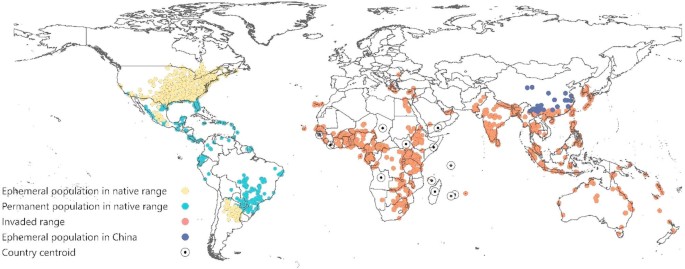
Confirmed presence records of Spodoptera frugiperda around the globe. Yellow occurrence records represent seasonal FAW populations within the native range. Light blue occurrence records show established FAW populations within its native range. Red occurrence records depict FAW populations within its invasive range. Dark blue occurrence records show the transient FAW populations based on population limits presented by Huang et al.65. Lastly, circled dots represent the centroid of a country/region (Angola, Yemen, Chad, Guinea-Bissau, Liberia, Madagascar, Mauritius, Mayotte, Réunion, Seychelles, Somalia, South Sudan), where FAW’s presence is confirmed only by a country centroid. This figure was created with QGIS version 3.36.2 (https://qgis.org/).
Climate data
We used the ‘CliMond CM_TC10: World’ climatology (C. Duffy, unpublished data) to fit the current climatic suitability of FAW under a rainfed and irrigation scenario. This dataset is interpolated in a 10-arc-minute gridded spatial resolution and consists of 30-year averages centred on 1995 (1981–2010) for daily minimum and maximum temperature (°C), monthly precipitation (mm), and relative humidity (%) recorded at 09:00 and 15:00 h. Additionally, we compared the CLIMEX output using the 1995-centered climate dataset with an equivalent one centred on 1975 (1961–1990), which is commonly used in CLIMEX studies (Figs. S2 – S3). Given climate change, an updated climate dataset representing the current climatic conditions could mean increased accuracy of the model outcomes.
Modelling package and softwareThe CLIMEX model
CLIMEX (Hearne Scientific Software, Melbourne66,67 is a process-based climatic niche model that allows the estimation of the potential distribution of species as a response to the current or future climate. It incorporates parameters pertaining to how a species’ development is affected by climatic conditions, offering a comprehensive understanding of the pest’s ecological niche. Several suitability indicators are calculated for each pixel/unit area by incorporating occurrence data and information on climatic parameters and species-specific ecophysiological growth parameters. The model is based on the assumption that a species’ population experiences one or more (un)favourable periods for growth in a given year67,66. During the favourable season in a given location, the weekly temperature and soil moisture requirements for population growth are met, as described by the annual Growth Index (GIA). In contrast, an unfavourable season is characterized by population decline and no growth and can be characterized using a selection of up to four stress indices (cold, hot, dry, wet) and four stress interaction indices (cold-dry, hot-dry, cold-wet, and hot-wet). Integrating the GIA and stress indices provides a single annual index of climatic suitability for a given location, the Ecoclimatic Index (EI). Both GIA and EI range from 0 to the theoretical maximum of 100. An EI value of 0 at a given location indicates that the species cannot persist year-round. In this study, we set a climatic suitability classification system for both EI and GIA, as follows: unsuitable for EI = 0, marginal for 0 30. We used the same classification system for every simulation, including the published CLIMEX models on FAW, to make the outputs comparable (Figs. S4, S5). QGIS (version 3.36.2) was used to project the CLIMEX output(s) and to visualize the different EI and GIA classes for FAW.
Table 1 CLIMEX parameter values used for modelling the Climatic suitability of Spodoptera frugiperda, based on five published studies and the current study.Model fitting
The climatic suitability of FAW was projected by using the “Compare Location (one species)” module in CLIMEX (version 4.1.1.0)67. We chose the set of CLIMEX parameter values for FAW of the most recently published model45 as a starting point. These parameter values were revised by considering (i) recent literature not used in previous CLIMEX models on climatic requirements for the growth and development of FAW, (ii) additional FAW global occurrence records, and (iii) other published CLIMEX models on FAW41,44,45,46,47. The model fitting was an iterative process. The main goal was to fit the model to the occurrence records representing permanent FAW populations, in regions where the limits of such populations are known, in the area with positive EI (EI > 0). We then confirmed that the occurrence points representing transient populations were within areas where the model indicates positive GIA (GIA>0) and EI = 0. FAW transient points in Fig. 1 are based on known permanent-transient population boundaries in the Americas and Canada68, and by Huang et al. in China65. It was not possible to accurately set permanent FAW population limits in southern Africa, Australia, and New Zealand due to insufficient data. In addition to fitting the distribution data, parameter values were also required to be biologically plausible. We compare the parameter values of the current study with those reported in five published CLIMEX models on FAW in Table 1. Further details and justification for the parameter values used in this study are discussed below.
Growth indicesTemperature index (TI)
Senay et al.46 chose a lower temperature threshold for development (DV0) of 8.7 °C as the minimum threshold for development averaged across all life stages of FAW, a result based on a second-degree polynomial regression69. However, because pupation is required to reach the sexually mature adult life stage and complete a generation, we used 9.4 °C as DV0, corresponding to the minimum temperature threshold for FAW pupal survival (same study69. The chosen DV0 value is similar to the field findings by Yang et al.70, who showed that FAW pupae can overwinter in the northern limit of Kunming in January 2020, where the average monthly temperature was 9.24 °C. Following the parameter values selected by du Plessis et al.71, the temperature range for optimal development was set from 26 °C (lower threshold—DV1) to 30 °C (upper threshold—DV2). and supported by more recent data on temperature-dependent development and survival rates72,73. According to Valdez-Torres et al.69, the maximum temperature threshold for FAW is 39.8 °C, thus the upper temperature for development (DV3) was rounded to 39.5 °C.
Moisture index (MI)
Recent experiments indicated that approximately 30% of FAW larvae burrowing in soil with 0% soil moisture were able to pupate successfully74. However, host plants cannot tolerate a complete absence of soil moisture, so we set the lower soil moisture threshold (SM0) at 0.1. The lower optimal soil moisture (SM1) was adjusted to 0.65, as FAW is highly polyphagous, and many plant species grow well at low moisture levels. The upper optimal soil moisture (SM2) and the upper soil moisture threshold (SM3) remained unchanged from the majority of previous CLIMEX models at 1.5 41,45,46 and 244, respectively. This allowed growth in the wettest areas of FAW’s distribution.
Stress indicesCold stress (CS)
FAW potential distribution appears sensitive to the cold stress parameters. The cold stress temperature threshold (TTCS) was set to 9.4 °C, in line with recent data supporting that FAW survival at different development stages decreases significantly when exposed to temperatures below 9 ± 0.5°C75,76,77. The cold stress accumulation rate (THCS) was adjusted to -0.003 week− 1 to allow FAW development in the cooler limits of its permanent populations2. Specifically, this included records along the Nile River Basin in Egypt, the Mediterranean coast of northern Africa, close to the border of Niger and Nigeria, north Argentina, the Australian state of Queensland, and southern China.
Heat stress (HS)
The heat stress temperature threshold (TTHS) was set to 39.5 °C, which is the value for DV3. The heat stress accumulation rate (THHS) was set to a moderate level of 0.005 week− 1 following du Plessis et al.41 and Senay et al.46. This allowed persistence in the hottest areas of FAW’s range.
Dry stress (DS)
The soil moisture dry stress threshold (SMDS) was set to 0.1, which is the value for SM0. The dry stress accumulation rate (HDS) was then adjusted to -0.005 week− 1 to limit the suitability projections to the tropical and subtropical areas where permanent FAW populations occur. This is also in agreement with most published CLIMEX models on FAW41,44,45,46.
Wet stress (WS)
The soil moisture wet stress threshold (SMWS) was set to 2 to be consistent with the value of SM3. Then, in accordance with Timilsena et al.44, the wet stress accumulation rate (HWS) was set to 0.01 week− 1 to restrain FAW suitability to the wetter tropical and subtropical regions where its permanent populations occur.
Minimum degree day sum (PDD)
This parameter describes the minimum required number of growing degree days above DV0 to complete a generation. Based on du Plessis71 estimates, FAW needs 391.61 °C days for egg-to-adult development. We rounded this parameter value to the nearest whole number (392 °C days) since CLIMEX is insensitive to such precision.
Irrigation
To account for irrigation, we ran the CLIMEX model with an irrigation scenario applied as an additional 2.5 mm day− 1 as a top-up above the default rainfed scenario, throughout the year. The Global Map of Irrigated Areas (GMIA) is used to define where the irrigation scenario shall be applied78. This assumes that no irrigation was added in areas where the rainfall is already equal to or greater than 2.5 mm day− 1, under the rainfed scenario. In the case of FAW, dry areas in North Africa, such as the Nile River, and in Pakistan and Yemen, where FAW occurs permanently and irrigation is applied, do not appear as climatically suitable under rainfed conditions44, supporting the hypothesis that they are able to persist in these locations only due to the presence of irrigation.
Modelled migration distances in Europe
FAW regularly migrates long distances during spring and summer. In North America, transient occurrence records have demonstrated the pest’s dispersal throughout the USA and southern Canada, causing substantial seasonal damage12,68. The spatial pattern of this seasonal dispersal was estimated using a subset of the original distribution dataset (n’=1 831) that consists of the transient occurrence records in the USA and Canada. These records are characterized by EI = 0 and GIA>0 in the afore-described CLIMEX model. Thus, we assessed the minimum distance of each transient occurrence point from the nearest area (hub) suitable for year-round population persistence (EI > 0; southern coast of the USA). Weinberg et al.79 employed a similar method to estimate the spatial pattern of seasonal dispersal of the southern armyworm (Spodoptera eridania). The QGIS “Distance to nearest hub (line to hub)” algorithm was used to compute the distance between each transient occurrence record and the closest destination layer (EI > 0 zone).
To reduce overestimation bias in our analysis, we excluded 115 occurrence records from the initial data subset (n = 1 946) because they were located on Bermuda Island (EI > 0). Including these records would imply that FAW flew more than 1 000 km overseas in a single event. The resulting dataset provided the distribution of minimum distances between transient FAW records and the nearest permanent establishment hub (EI > 0). Based on this distribution, we created buffer zones around the modelled EI > 0 area (hub)79. These buffer zones represent dispersal frequency zones and illustrate areas that may be accessible to FAW transient populations, with the risk of migration diminishing as the distance from the EI > 0 area increases (Fig. S6). For instance, Fig. 3 shows two buffer zones derived from the 50th and 100th percentile of the FAW migration distances distribution, indicating median and maximum potential extents of FAW natural migration, at least under average climatic conditions. A GIA>0 area that falls adjacent to, or within these buffer zones, indicates potential crop exposure to migrating populations. Conversely, GIA>0 areas outside the buffer zone of maximum distance are assumed to be inaccessible to FAW by flight.
Assuming that FAW observed migratory capacity in Europe is broadly similar to its behaviour in its native range, we applied these dispersal frequency zones across the European continent. The results were considered alongside our CLIMEX model outcomes, which identify climatically suitable areas for seasonal FAW populations (GIA>0) within Europe.
Direct economic impactEconomic data
National average values of grain maize revenues and operating costs from 2010 to 2020 were obtained from the EU Cereal Farms database of the Farm Accountancy Data Network (FADN) for 13 EU MSs: Austria, Bulgaria, Croatia, France, Germany, Greece, Hungary, Italy, Poland, Portugal, Slovakia, Slovenia, and Spain. We also used EUROSTAT to obtain information on the grain maize cultivated area for each MS. These MSs contributed more than 80% of the total grain maize production in the EU-27 for the years 2022 and 2023, respectively (own calculation based on EUROSTAT). Moreover, the European Food Safety Authority (EFSA) provides expert-elicited estimates on grain maize yield losses due to FAW, based on formal EKE methodology80,81,82. In the case of grain maize, losses are the consequences of plant decline and rejected, and unharvested cobs. A key assumption of the EKE data is that similar levels of yield loss occur in both permanent and transient FAW population areas.
Direct economic impact
To estimate the direct economic impact of FAW invasion on European grain maize production, we employed a partial budgeting method. Partial budgeting is an appropriate method to evaluate the economic consequences of a shock, such as a pest invasion, by accounting for the potential economic benefits and losses57. In the case of FAW, direct impacts include solely negative effects, namely yield losses and additional operating costs. The direct economic impact was estimated over the study area where the CLIMEX model projected the establishment of FAW (Mediterranean coast) but was limited to where the migratory behaviour and capacity analysis suggested the likelihood of seasonal populations. However, this encapsulated all of the 13 EU MSs included in the FADN dataset. We performed the analysis under the irrigation scenario since it better reflects FAW’s ecological niche. Furthermore, the baseline grain maize gross margins were computed and compared with the gross margins with FAW presence.
The direct economic impact assessment was conducted under specific assumptions. Firstly, we performed the analysis under a post-invasion no-control scenario83, assuming that no additional regulatory or control measures are in place after the invasion, and thus no change in the operating costs. This “worst-case” scenario provides a benchmark for the potential scale of damages due to FAW without intervention. Secondly, we also assumed a complete occupancy of the climatically suitable area (EI > 0) in Europe (Mediterranean coast) and that the northward migration starts over from that area each year. This assumption aligns with the pest’s observed behaviour in its native (and invaded) range, where areas with permanent FAW populations serve as sources for seasonal dispersal. Thirdly, the migratory capacity of FAW follows a similar pattern as in the USA and Canada, thus, the representation of accessible zones outside the area of permanent establishment remains consistent in Europe. Fourthly, the probability of attack is inversely related to the distance from the permanent FAW establishment area, reflecting the diminishing annual likelihood of successful migration as distance increases. Therefore, northern EU MSs bear a smaller risk than those further south. Finally, the economic model only accounts for the natural migration of the pest through flight; other dispersal pathways, such as trade, were not considered in the analysis.
Baseline gross margins
We used the gross margin per hectare (€/ha) as a baseline representing the current economic state of EU grain maize in each MS. Gross margins capture the difference between revenue and operating costs, providing a more accurate reflection of farm-level profitability than just revenues alone. The gross margin is calculated as follows:
$$GM_{i}^{{baseline}} = \frac{1}{n}\sum {\:_{{t = 1}}^{n} } (R_{{i,t}} – OC_{{i,t}} )$$
(1)
\(\:{GM}_{i}^{baseline}\) is the average grain maize gross margin per hectare (€/ha) which is determined by the difference between annual revenues per hectare \(\:{R}_{i,t}\) and operating costs per hectare \(\:{OC}_{i,t}\) in each MS \(\:i\) and for each year \(\:t\) over the period 2010–2020. The \(\:{OC}_{i,t}\) component takes into account several cost categories, such as specific costs (€/ha) (seeds, fertilizers, crop protection, water, other specific costs) and non-specific costs (€/ha) (motor fuels and lubricants, machines, buildings, contract work, energy (electricity, heating fuels) and other direct costs).
Gross margins with FAW
The gross margins under FAW presence represent the post-invasion grain maize gross margins were calculated as:
$$\begin{array}{*{20}c} {GM_{i}^{{FAW}} = \bar{R}_{i} \left( {1 – PP_{i} \frac{{YL_{{i,s}} }}{{100}}} \right) – \overline{{OC}} _{i} } \\ \end{array}$$
(2)
\(\:{GM}_{i}^{FAW}\)is the grain maize gross margin with FAW presence in MS \(\:i\) (€/ha), \(\:{\stackrel{-}{R}}_{i}\) and \(\:{\stackrel{-}{OC}}_{i}\) are the average revenue and operating costs (€/ha) in MS \(\:i\), respectively, \(\:{YL}_{i,s}\) is the EKE yield loss for MS \(\:i\) and yield loss scenario \(\:s\), and \(\:{PP}_{i}\) is the probability of FAW presence for MS \(\:i\).
The \(\:{PP}_{i}\) parameter accounts for each MS’s annual risk of invasion based on its geographical proximity to areas of FAW establishment (EI > 0). We assume that northern countries face lower risks compared to those located in the south, which are closer to the area of permanent establishment. More specifically, \(\:{PP}_{i}\) captures the probability of FAW presence in a MS, considering the pest’s migratory capacity (flight distance), whereas \(\:{YL}_{i,s}\) incorporates the expert-elicited yield losses82 that may be affected by several factors, including FAW population abundance and short generation time (Table S1).
To estimate the \(\:{PP}_{i}\) for each MS \(\:i\), we used an empirical cumulative distribution function (ECDF). We utilized the data subset that includes the distance distribution of transient FAW occurrence records in North America. An ECDF value represents the proportion of all observed migration distances that are less than or equal to a specific distance away from the projected area of permanent FAW establishment. Thus, ECDF allows us to assign a probability to a specific distance of interest from the EI > 0. The \(\:{PP}_{i}\) parameter is calculated as:
$$\begin{array}{*{20}c} {PP_{i} = 1 – F\left( {D_{i} } \right)} \\ \end{array}$$
(3)
where \(\:{D}_{i}\) denotes the distance from the centroid of MS \(\:i\) to the nearest area with EI > 0 along the Mediterranean coast and \(\:F\left({D}_{i}\right)\:\in\:\left[\text{0,1}\right]\) is the ECDF value at that distance. This approach assumes the inverse relation between distance and invasion risk with proximity to EI > 0 corresponding to higher risks of FAW invasion (Figs. S7, S8).
To extend the per-hectare direct impacts (€/ha) to national levels, we scaled the per-hectare gross margins by the total cultivated area of grain maize in each MS. In particular, we multiplied the gross margins (€/ha) by the total grain maize cultivation area, based on EUROSTAT data from 2013 to 2023, for each MS.
Lastly, the direct economic impact \(\:{DEI}_{i,s}\) is calculated by comparing the baseline gross margins to those under FAW presence:
$$\begin{array}{*{20}c} {DEI_{{i,s}} = GM_{i}^{{baseline}} – GM_{{i,s}}^{{FAW}} } \\ \end{array}$$
(4)
Three scenarios were considered to capture the bandwidth of the potential impact of FAW on European grain maize production: a best-case, moderate-case, and worst-case scenario that assume a yield loss percentage equal to the 2.25th, 50th, and 97.5th percentiles of the MS-specific yield loss distribution, respectively. These yield loss scenarios are based on the EFSA EKE data80,81,82, which incorporate various assumptions, including the effectiveness of current, untargeted control measures against FAW, climate conditions, and damage type. One example of such indirect management is the chemical control against Helicoverpa armigera, which may also have a collateral benefit tackling FAW populations84. Table S1 provides the reasoning behind each scenario, and Table S2 includes the exact values.