Data compilationData sources
We gathered data on IWT incidents occurring via the flight network from two of the most expansive resources on IWT activity. The first is from ROUTES, a conglomerate of transit companies, government agencies, conservationists, law enforcement, and academics working to address global wildlife crime39. Their corresponding airline traffic database contains data on 975 unique trafficking incidents on the airline network between 2010 and 2020. The second resource comes from TRAFFIC, a global NGO focused on ensuring the wildlife trade is both legal and sustainable40. They created the Wildlife Trade Portal, an online portal that allows users to query for wildlife seizure data and filter by location, species, transportation type, and time41. The Wildlife Trade Portal is not exclusive to just incidents occurring on the flight network, so we filtered for incidents with at least one documented location occurring at an airport by gathering all incidents with Airport listed in the Transit Type column. As TRAFFIC was a member of the ROUTES partnership, we only counted incidents occurring after 2020 to avoid double-counting. TRAFFIC yielded 346 incidents between 2021 and 2023, totaling 1321 incidents.
Building the full flight network
To build the full flight network consisting of all airports and flights available across the globe, not just those with observed trafficking activity, we collected data from OpenFlights.org, which hosts open-source information on airports and flights available globally42. Any references to an airport’s centrality in the full flight network were calculated using the equations in Section “Centrality Calculations” using all 1933 airports/nodes and 14,118 flights/edges. Importantly, this database is not updated instantaneously when new flight routes begin. Therefore, after verifying the flight existed by searching Google Flights, we manually added a small number of routes present in our dataset of 1.3K IWT incidents. This ensures the maximum number of IWT records were captured and that the IWT flight network is a proper subgraph of the full flight network.
Building the IWT flight network
To build the IWT flight network, we used a subset of the 1321 IWT incidents. We filtered the 1321 incidents for those with at least two documented stops at airports. This was done to ensure the edges strictly represented flights between two airports involved in the IWT. The size of the resulting dataset consisted of 478 distinct incidents, showcasing the completeness bias of the dataset. Any references to an airport’s centrality in the IWT network were calculated using the airports and flights observed in the 478 incidents using the equations in Section “Centrality Calculations”.
Centrality calculationsDegree centrality
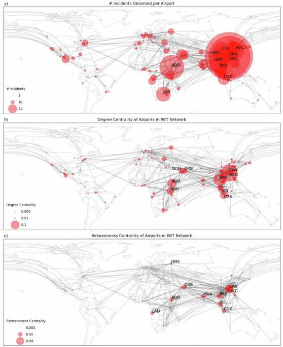
Degree centrality equals the number of edges connected to a node21. In the full flight network, it represents the number of direct flights into or out of a given airport. In the IWT flight network, degree centrality represents the number of direct flights into or out of airports with documented IWT activity. Airports with high degree centrality are crucial in both the full flight network and IWT networks, as they connect to many other airports, playing a vital role in the movement and distribution of IWT. We calculated degree centrality of airports in both the full flight and IWT networks using the NetworkX package in Python, which normalizes the centrality to values between 0 and 1 using Eq. (1).
$${C}_{{\rm{degree}}}(v)=\frac{ {\text{degree}} \, {\text{of}} \, {\text{node}} \, v} { {\text{total}} \, {\text{number}} \, {\text{of}} \, {\text{nodes}} \,-1}$$
(1)
Betweenness centrality
Betweenness centrality equals the number of shortest paths a given airport is on between any two airports in a network22. Airports with high betweenness centrality are crucial connection points or bridges between origin and destination airports. We calculated the betweenness centrality of airports in both the full flight and IWT networks using the NetworkX package in Python, which normalizes the centrality to values between 0 and 1 using Eq. (2).
$${C}_{{\rm{betweenness}}}(v)=\sum _{s\ne v\ne t}\frac{{\sigma }_{st}(v)}{{\sigma }_{st}}$$
(2)
where σst is the number of shortest paths between source s and target t and σst(v) are those that pass through node v.
Predictive model formulationFeature overview
We considered 44 features of the airports in four different categories: location, the presence of criminal markets, criminal actors, and counter-crime resilience measures.
Features that fall under location metadata include the population of the city the airport is located in and whether the country is a member of CITES (the Convention in International Trade in Endangered Species of Wild Fauna and Flora, a nonbinding agreement to protect endangered plants and animals from the threats of international trade)43. We collected data on whether a country was a signatory of CITES from 2016 to 2021. Location metadata also includes centrality measures for the airports and their positions in the full flight network, using the data gathered in Section “Data Compilation”. We only included centrality metrics of the full flight network because the label we aimed to predict was participation in IWT. Therefore, adding features that rely on knowing IWT participation induces a circular process. The features in the three other categories originate from the 2021 Global Crime Index, measured by the Global Initiative against Transnational Organized Crime (GITOC). This organization provides numerical scores on a country’s criminal market, criminal actors, and resilience measures. The features in these areas are intended to quantify the levels of organized crime in a country and assess their resilience to organized criminal activity28. Each country’s value is evaluated over two years and draws from both quantitative and qualitative sources. The final scores are decided by 400+ experts and GITOC’s regional observatories. All features and their subsequent values were normalized to values between 0 and 1.
These categories of features were selected based on prior works that highlight the convergence of multiple forms of illicit trade4,44. Because little data is available on wildlife trafficking, more well-researched illicit networks, such as drug and human trafficking, can lend insights into how wildlife traffickers operate. GITOC gathers this data and categorizes the features into three groups: criminal actors, criminal networks, and resilience. We considered all feature categories in our model. The last category, location, was included to highlight the centrality measures we gathered as well as other location-specific features we hypothesized could hold predictive power of IWT involvement (i.e., CITES membership and population).
Our dependent variable, IWT participation, is a binary representation of whether the airport was observed to have IWT activity in the dataset of 1.3K incidents described in Section “Data Compilation”. Our dataset exhibited significant class imbalance, with only 311 (16%) airports having observed IWT activity and the remaining 1622 having no documented IWT activity.
Full descriptions of all the features used in modeling can be found in Supplementary Data 1.
Feature selection
To improve the performance of our predictive model, we completed two feature reduction measures. The first was removing features that were highly correlated with one another to reduce the risk of overfitting and increase model interpretability45,46,47. To determine which features to remove, we ranked features by their Pearson correlation with the dependent variable, IWT participation, using the pearsonr function from the scipy.stats Python library. We then iteratively eliminated those with a correlation above 0.80 with more significant features. This process removed 13 features.
With the initial reduction of features complete, we trained and tested a series of models to select the best-performing one with the remaining 31 features. Using the optimal model, we then conducted both forward and backward feature selection on the remaining features to identify which method maximized the model’s ROC-AUC Score48,49. Backward feature selection works by starting with all available features and progressively eliminating the feature that, when excluded, results in the highest ROC-AUC score for the remaining set until the target number of features is met. Forward feature selection works by starting with an empty set of features and adds them one-by-one, selecting the feature that, when included, produces the highest increase in the ROC-AUC score until the target number of features is met. To limit computational resources, we attempted both methods, specifying that either 5, 10, 15, 20, 25, or 30 variables were selected, picking whichever variable count yielded the highest ROC-AUC score. Using the final variable count output in that process, we then utilized a sequential process of choosing which variables to include by maximizing the ROC-AUC score at each variable addition. We used 5-fold cross-validation to evaluate performance across all data points at each iteration. Backward feature selection returned both the maximum ROC-AUC and class-weighted F1 score of the two methods when utilizing ten features, so we proceeded with modeling using features the following features: betweenness centrality, degree centrality, non-state actors, territorial integrity, non-renewable resource crimes, floral crimes, foreign actors, prevention, political leadership and governance, and human trafficking.
Model selection & execution
We attempted multiple classification models, including logistic regression, decision trees, random forests, balanced random forests, gradient boosting machines, and linear discriminant analysis, using SMOTE oversampling where appropriate, and 5-fold cross-validation to evaluate performance. We prioritized traditional machine learning methods over black-box models as conservation practitioners highlight the importance of adopting interpretable methods to understand, in our case, why wildlife trafficking occurs at some locations over others50,51,52. All modeling techniques were executed using Python and its various libraries. We used 5-fold cross-validation to evaluate each model’s performance at testing to ensure each data point was evaluated53. The balanced random forest model achieved the highest ROC-AUC and class-weighted F1 score, so we proceeded with this model utilizing imbalanced learn’s ensemble.BalancedRandomForest package54.
Classical random forests can be biased towards the majority class where significant class imbalance exists, such as our dataset where only 311 (16%) airports were observed with IWT activity26. Balanced models can better handle imbalanced datasets, specifically reducing bias towards the majority class using bootstrapping, meaning the number of samples drawn from each class is the same, ensuring the minority class is represented in each tree26. Using a balanced model in our study methods allows us to extract information from the few positive samples in our dataset to make inferences on.
We also performed hyperparameter tuning, though we proceeded with default parameters as performance changes were negligible. Supplementary Table 1 showcases the ROC-AUC scores of each model’s performance with the 31 features remaining after the correlation analysis removed 13 features discussed previously, as well as the best-performing model after conducting BFS and FFS – the balanced random forest model with 10 features selected with BFS. To showcase performance improvements due to removing highly correlated variables, we also reported the ROC-AUC score of the balanced random forest using all 44 variables.