This section proposes a decision procedure based on fuzzy logic to distribute jobs between the fog and cloud layers. It also presents a real-time task scheduling mechanism to select the most suitable virtual machine for task execution. There are two stages involved in implementing the suggested method, Dynamic Task Allocation in Fog Computing Using Fuzzy Logic Enhanced (DTA-FLE). First, using a task categorization technique based on fuzzy logic, the tasks are assigned to LCFL, HCFL, and CL. Second, the DTA technique is used to plan the tasks inside each layer. Algorithm 1 provides pseudo code of the proposed method. Meanwhile, Table 2 shows a summary of the notations used in this study.
Algorithm 1
DTA-FLE (Dynamic Task Allocation using Fuzzy Logic Enhanced).
Table 2 Notations used in this study.Fuzzy logic-based task scheduling mechanism
Based on the resource requirements of each task, time constraints, the maximum available resources in the fog layer, and the latency between the fog and cloud layers, the fuzzy decision-making algorithm determines whether a given task should be processed in the fog or offloaded to the cloud. If task ti is selected to be executed in the fog layer, the algorithm computes the normalized minimum resource requirements for CPU, storage, and bandwidth. These normalized values help evaluate the feasibility of executing the task locally in the fog. Specifically, if task \(\:{t}_{i}\) is assigned to the fog, the minimum values of the task’s resource consumption needs, in terms of CPU rate \(\:{c}_{\text{m}\text{i}\text{n}}\left({t}_{i}\right)\), storage \(\:{s}_{\text{m}\text{i}\text{n}}\left({t}_{i}\right)\), and bandwidth \(\:{b}_{\text{m}\text{i}\text{n}}\left({t}_{i}\right)\), are as follows:
$$\:{c}_{min}\left({t}_{i}\right)=\frac{ct\left({t}_{i}\right)}{c{c}_{max}v},\:{s}_{min}\left({t}_{i}\right)=\frac{st\left({t}_{i}\right)}{s{c}_{max}v},\:{b}_{min}\left({t}_{i}\right)=\frac{bt\left({t}_{i}\right)}{b{c}_{max}v}$$
(1)
where \(\:ct\left({t}_{i}\right)\) represents the required CPU cycles (processing capacity) for task \(\:{t}_{i}\), \(\:st\left({t}_{i}\right)\) represents the required storage space for task \(\:{t}_{i}\), and \(\:bt\left({t}_{i}\right)\) represents the required bandwidth for data transmission associated with task \(\:{t}_{i}\). Also, \(\:c{c}_{\text{m}\text{a}\text{x}}v={\text{m}\text{a}\text{x}}_{{v}_{j}\in\:V}\:cc\left({v}_{j}\right)\:\)represents the maximum CPU rate that the fog layer offers. Similarly, the maximum bandwidth and storage capacity in the fog layer are denoted by \(\:b{c}_{\text{m}\text{a}\text{x}}v={\text{m}\text{a}\text{x}}_{{v}_{j}\in\:V}\:bc\left({v}_{j}\right)\) and \(\:s{c}_{\text{m}\text{a}\text{x}}v={\text{m}\text{a}\text{x}}_{{v}_{j}\in\:V}\:sc\left({v}_{j}\right)\), respectively.
Fuzzy sets for input and output parameters are used in fuzzy logic systems to represent uncertain or imprecise information. For input parameters, a fuzzy set assigns a degree of membership between 0 and 1 to each possible value, indicating how strongly it belongs to the set. Similarly, for output parameters, fuzzy sets help determine the degree to which a particular outcome is associated with the given input conditions. This approach allows for more flexible and human-like reasoning, especially in complex or ambiguous environments where traditional binary logic falls short. The fuzzy sets for the input and output parameters are described in Table 3. Meanwhile, Fig. 2 shows the membership functions of the input and output fuzzy set variables.
Table 3 Fuzzy input/output variables along with desired fuzzy sets.
Using Eqs. (2–6), the membership values for the fuzzy input parameters are computed. These equations define triangular and trapezoidal membership functions, which are common in fuzzy logic systems for representing uncertainty and linguistic terms (e.g., low, medium, high). In all equations, \(\:\mu\:\left(x\right)\) denotes the membership value, which is a real number in the interval [0,1]. It represents the degree to which the input \(\:x\) belongs to a particular fuzzy set. Also, x represents the crisp input value, i.e., the actual numerical value of a parameter (such as latency, cost, etc.).
$$\:\mu\:\left(x\right)=\left\{\begin{array}{ll}0,&\:x>0.5\\\:\frac{0.5-x}{0.5-0.2},&\:0.2\le\:x\le\:0.5\\\:1,&\:x
(2)
$$\:\mu\:\left(x\right)=\left\{\begin{array}{ll}0,&\:x\le\:0.2\\\:\frac{x-0.2}{0.5-0.2},&\:0.2
(3)
$$\:\mu\:\left(x\right)=\left\{\begin{array}{ll}0,&\:x0.8\end{array}\right.$$
(4)
$$\:\mu\:\left(x\right)=\left\{\begin{array}{ll}0,&\:x>0.6\\\:\frac{0.6-x}{0.6-0.4},&\:0.4\le\:x\le\:0.6\\\:1,&\:x
(5)
$$\:\mu\:\left(x\right)=\left\{\begin{array}{ll}0,&\:x0.6\end{array}\:\right.\text{\:Cloud\:Layer}$$
(6)
Fig. 2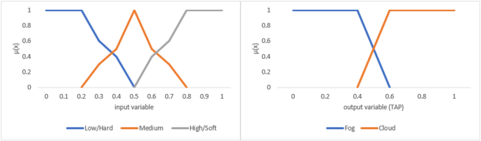
Membership functions of the Input and Output fuzzy set variables.
Using experimental data, we have created a fuzzy logic rule base of 243 rules based on five input and one output variables. Table 4 presents a sample of the rule base41. Because of its ease of use, the Mamdani Fuzzy Inference System (MFIS) has been adopted42,43. The enter of Gravity (CoG) defuzzification method is used to convert the output fuzzy sets into a single crisp value once the fuzzy output has been produced in accordance with the criteria.
Table 4 Defined set of fuzzy rules.
Let’s consider a practical example where a task requires scheduling in a fog computing environment. Suppose we have a task \(\:{t}_{i}\) that needs to be executed, and it requires 50 CPU cycles, 100 MB of storage, and 20 Mbps of bandwidth. The fog layer provides VMs with varying available resources, and we need to decide whether this task should be processed in the fog or offloaded to the cloud. First, using the fuzzy logic-based scheduling mechanism, we compute the normalized minimum resource requirements for the task based on the available resources in the fog layer. Let’s assume the maximum available CPU rate in the fog layer is 200 CPU cycles per VM, the maximum storage is 500 MB, and the maximum bandwidth is 100 Mbps. Using the normalization formulas for CPU, storage, and bandwidth, we calculate:
$$\:{c}_{min}\left({t}_{i}\right)=\frac{50}{200}=0.25,\:{s}_{min}\left({t}_{i}\right)=\frac{100}{500}=0.2,\:{b}_{min}\left({t}_{i}\right)=\frac{20}{100}=0.2$$
Next, we evaluate the fuzzy membership values for the task’s resource utilization (CPU, storage, bandwidth), deadline, and network latency using fuzzy sets defined in Table 3. For instance, if the task’s latency is low, the deadline is hard, and resource utilizations are low, we determine that the task belongs more strongly to the “Fog Layer” fuzzy set based on the membership functions and rule base provided. Finally, after applying the fuzzy decision-making algorithm, the task is assigned to the fog layer as it meets the resource requirements for local execution. The fuzzy inference system uses the computed membership values and rules to decide the most suitable layer (fog or cloud) for task execution based on real-time conditions, such as latency, resource utilization, and deadline constraints.
Task scheduling technique
Tasks that arrive at the fog broker are queued \(\:Q\) and handled by the suggested Fuzzy Logic-based Real-time Task Scheduling Algorithm. The task is sent to the cloud if the fog layer is unable to supply the resources needed for it. If not, the min-max normalization is used to calculate and normalize the task’s minimum resource consumption needs. The Fuzzy Logic-based Decision Algorithm is employed to determine if a job should be processed on the fog or forwarded to the cloud, taking into account the task’s resource consumption, deadline, and network latency. The job is added to a fog queue \(\:FQ\) if it is assigned to the fog layer. The deadlines of each work are arranged in ascending order within the fog queue. This ensures that more tasks are finished by the deadline by processing the urgent ones with strict deadlines first. Next, by examining each virtual machine’s eligibility, a collection of \(\:{V}^{{\prime\:}}\)eligible virtual machines (VMs) are generated for every task. Among the VMs \(\:{v}^{{\prime\:}}\) that meet the eligibility requirements, the one with the least amount of load is chosen, and it is given the assignment. To assess the performance and efficiency of task allocation in a fog computing environment, it’s essential to evaluate how well a VM utilizes its allocated resources. The total resource utilization of a virtual machine \(\:{v}_{j}\) is calculated using the average of its individual resource utilizations—namely CPU, storage, and bandwidth:
$$\:ru\left({v}_{j}\right)=\frac{\left(cu\left({v}_{j}\right)\text{*}su\left({v}_{j}\right)*bu\left({v}_{j}\right)\right)}{3}$$
(7)
where \(\:ru\left({v}_{j}\right)\) represents the total resource utilization of VM \(\:{v}_{j}\), \(\:cu\left({v}_{j}\right)\) represents the CPU utilization of VM \(\:{v}_{j}\), \(\:su\left({v}_{j}\right)\) represents the storage utilization of VM \(\:{v}_{j}\), and \(\:bu\left({v}_{j}\right)\) represents the bandwidth utilization of VM \(\:{v}_{j}\). Meanwhile, \(\:u\left({v}_{j}\right)=\frac{\sum\:_{i=1}^{N}\:ct\left({t}_{i}\right)}{cc\left({v}_{j}\right)}\), \(\:su\left({v}_{j}\right)=\frac{\sum\:_{i=1}^{N}\:st\left({t}_{i}\right)}{sc\left({v}_{j}\right)}\) and \(\:bu\left({v}_{j}\right)=\frac{\sum\:_{i=1}^{N}\:bt\left({t}_{i}\right)}{bc\left({v}_{j}\right)}\). Here, \(\:cc\left({v}_{j}\right)\), \(\:sc\left({v}_{j}\right)\), and \(\:bc\left({v}_{j}\right)\) represent total available CPU capacity, total storage capacity, and total available bandwidth of VM \(\:{v}_{j}\), respectively. Also, \(\:N\) represents the total number of tasks.
We have three task queues after using the fuzzy-logic-based task scheduling technique. Every queue from HCFL, CL, and LCFL for every layer. DTA is carried out using a series of procedures that are described as follows, taking into account the queue of categorized tasks in the layer and the number of VMs in each processing server on that layer:
-
(1)
Calculate the Expected Processing Time (EPT) matrix for each task (\(\:i\)) on all VMs in each Processing Server (PS). As per Eq. (8), the size of the EPT matrix is determined by multiplying the number of tasks with the number of servers and the matching number of VMs. Depending on the VM’s processing power, a task’s EPT varies from one to the next. This equation calculates the expected time it would take for each task to execute on each VM across all processing servers. It allows the task scheduler to evaluate all potential task-to-VM assignments in order to choose the most efficient option based on processing time.
$$\:EPT(i,k,j)=\frac{TLength\left(i\right)}{VM\_MIPS\left(j\right)}$$
(8)
where \(\:i\) denotes the current task index, \(\:k\) denotes the current PS index, and \(\:j\) denotes the VM index within that \(\:k\)-th PS. Also, \(\:EPT(i,k,j)\) denotes the EPT of \(\:{t}_{i}\) on \(\:{v}_{j}\) that resides within \(\:{p}_{k}\).
-
(2)
Assigning a task to the VM with the freest time and the lowest EPT. The task with the shortest maxRT is assigned first. Suppose task \(\:{t}_{i}\) requires scheduling. The objective is to assign it to a VM in a manner that minimizes its completion time. To achieve this, the Expected Time to Completion (ETC) is calculated for all possible combinations of processing sites and VMs. The combination with the lowest ETC value—indicating the earliest expected finish time—is then selected for task assignment. Equation (9) calculates the ETC for assigning task \(\:{t}_{i}\) to VM \(\:{v}_{j}\) in a processing site \(\:{p}_{k}\).
$$\:ETC\left(k,j\right)=wt\left(k,j\right)+EPT\left(i,k,j\right)$$
(9)
where \(\:EPT(i,k,j)\) is the task’s estimated processing time and \(\:wt(k,j)\) is the processing time for the VMs availability. Meanwhile, \(\:ETC\left(k,j\right)\) represents the total expected time to complete task \(\:{t}_{i}\) on VM \(\:{v}_{j}\) in processing site \(\:{p}_{k}\), considering both the waiting time for the VM and the estimated processing time for the task.
-
(3)
Using Eq. (10), calculate the Total Expected Time to Complete (TETC) for task \(\:{t}_{i}\) on VM \(\:{v}_{j}\) in \(\:{p}_{k}\):
In Eq. (10), the Total Expected Time to Complete (TETC) for a task \(\:{t}_{i}\) on VM \(\:{v}_{j}\) in \(\:{p}_{k}\) is calculated as the sum of the ETC for the task and the transmission time \(\:{T}_{rans}^{s}\left(i\right)\). The transmission time accounts for the time required to transmit the task data to the processing unit, which is computed in Eq. (11)7.
$$\:TETC\left(k,j\right)=ETC\left(k,j\right)+{T}_{rans}^{s}\left(i\right)$$
(10)
$$\:{T}_{rans}^{s}\left(i\right)=\frac{TSize\left(i\right)}{BW}$$
(11)
where \(\:BW\) is the task classifier’s and the processing server’s link bandwidth, and \(\:TSize\left(i\right)\) refers to the size of the task data for task \(\:{t}_{i}\).
Practical applications
In the proposed DTA-FLE method, the system classifies tasks based on fuzzy logic and then schedules them in the most suitable VM within the fog or cloud layers. For instance, consider a task \(\:{t}_{i}\) with certain resource requirements, such as CPU, storage, and bandwidth. First, the fuzzy logic-based task classification evaluates these requirements and assigns the task to one of three categories: LCFL, HCFL, or CL. After categorization, the task enters the appropriate queue. Next, the DTA algorithm computes the EPT for each VM in each layer based on the task’s resource needs and the VM’s processing capacity. The task is then assigned to the VM with the least expected time to complete the task, factoring in both waiting time and processing time. Additionally, the method accounts for transmission time, which is the time needed to send task data across the network, using the bandwidth between the task classifier and the processing server. This comprehensive scheduling approach optimizes resource utilization, minimizes latency, and ensures that tasks are completed within their deadlines, thereby improving overall system performance.
In practical applications, the proposed DTA-FLE method can be particularly useful in scenarios where IoT devices are deployed across a wide geographic area, such as in smart cities or industrial automation. For example, in a smart city scenario, traffic monitoring tasks can be categorized based on their urgency and resource needs. High-priority tasks, such as detecting accidents or traffic jams, may be classified into the HCFL for immediate processing at nearby fog nodes, ensuring low latency. On the other hand, tasks like real-time weather updates, which have less stringent time constraints, may be assigned to the CL for processing, utilizing more computational power. Additionally, tasks like video surveillance may require substantial bandwidth and storage, so they are first evaluated by fuzzy logic and assigned to the most suitable VM based on available resources. This approach allows the system to dynamically balance the load between fog and cloud layers, optimizing resource allocation, minimizing latency, and ensuring that critical tasks are processed on time. Such a method is also applicable in industrial IoT, where machines and sensors continuously send data for analysis, and real-time task scheduling ensures smooth operation without delays or resource bottlenecks.
Experimental evaluation
This section estimates the performance metrics and provides the performance evaluation of the suggested DTA-FLE technique. Additionally, we evaluate the DTA-FLE approach’s performance in comparison to that of OEeRA15, FBOT20, and DTA. We have already deployed OEeRA, FBOT, and DTA in the identical DTA-FLE environment configuration to allow for a fair comparison.
According to their order of arrival, tasks are carried out on the fog-cloud servers via the OEeRA technique, with the first task to arrive being served first. Servers in the LCFL come first, followed by servers in the HCFL, and lastly, servers on the cloud layer. Tasks on the fog-cloud servers are carried out by the FBOT technique according to their lengths. According to length, the tasks are arranged in ascending order. The tasks are subsequently assigned to servers in LCFL, HCFL, and Cloud, in that order, much like in OEeRA. In DTA, tasks are arranged in ascending order according to their maximum response times, and only cloud servers are scheduled. The following metrics are calculated and explained in order to assess the suggested solution in line with OEeRA, FBOT, DTA, and DTA-FLE: makespan, energy consumption, cost of processing, guarantee ratio, and delay.
The suggested approaches are implemented and examined using the iFogSim simulator30. It is an open-source simulation toolkit based on Java that enables the evaluation of resource management and scheduling strategies across fog and cloud resources. The jFuzzylogic open-source Java library is used to link the fuzzy logic platform with iFogSim30. In this Task, the simulation parameters are as follows: The task length is set according to a random number between [1000 MI, 5000 MI]. The number of tasks is set between 100 and 700. Data size is set according to a random number between [10 KB, 500 KB]. MaxRT is set according to a random number between [3 s, 15 s]. The processing cost per time unit in the cloud is equal to 1$. The simulation parameters for tasks, servers, and VMs are listed in Table 5. We assume that each fog server has four VMs and each cloud server has ten VMs with varying computational capacity.
Table 5 Simulation parameters for VMs and servers7.
We evaluated the impact of increasing task counts from 100 to 700 on performance metrics, averaging outcomes over ten simulation runs.
Makespan
As shown in Fig. 3, the makespan increases with the number of tasks. DTA-FLE consistently shows a lower makespan compared to DTA, FBOT, and OEeRA. For instance, at 500 tasks, the makespan for DTA-FLE is 8.35 s, compared to 11.7 s for DTA, 44.41 s for FBOT, and 46.62 s for OEeRA. This means DTA-FLE executes tasks 81% faster than FBOT and OEeRA and 29% faster than DTA. DTA-FLE achieves this by prioritizing urgent tasks with shorter maximum response times, allocating them to hierarchical fog levels, and directing less urgent tasks to the cloud layer. This approach results in fewer tasks assigned to fog devices compared to FBOT and OEeRA, where more tasks are allocated to fog than to the cloud.
Fig. 3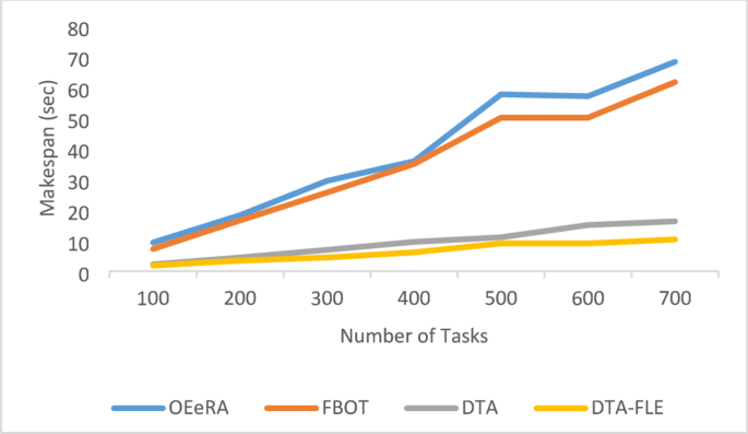
Effect of varying number of tasks on makespan.
Energy consumption
Energy consumption is a crucial factor in fog computing environments, as resource-constrained edge devices must operate efficiently while processing tasks. To evaluate the effectiveness of our proposed approach, we compared its energy consumption against three existing methods: DTA, FBOT, and OEeRA. Energy consumption in our study is calculated based on the total power usage of fog nodes and cloud servers during task execution. The power model considers both computation energy (\(\:{E}_{comp}\)) and communication energy (\(\:{E}_{comm}\)), formulated as follows:
$$\:{E}_{comp}=\sum\:_{i=1}^{n}{P}_{CPU}*{T}_{exec}$$
(12)
$$\:{E}_{comm}=\sum\:_{i=1}^{m}\left({P}_{tx}+{P}_{rx}\right)*{T}_{comm}$$
(13)
where \(\:{P}_{CPU}\) is the power consumption of processing units, \(\:{T}_{exec}\) is the task execution time, \(\:{P}_{tx}\) and \(\:{P}_{rx}\) are the transmission and reception power, respectively, and \(\:{T}_{comm}\) is the communication time. Also, \(\:n\) and \(\:m\) are the number of tasks and the number of computing resources, respectively.
As depicted in Fig. 4, the proposed DTA-FLE approach achieves lower energy consumption across all task loads compared to DTA, FBOT, and OEeRA. This improvement is attributed to the intelligent task allocation mechanism of DTA-FLE, which minimizes unnecessary task migrations and optimizes resource utilization within the fog layer.
Fig. 4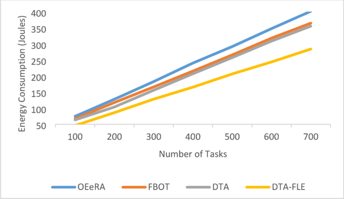
Effect of varying number of tasks on energy consumption.
Cost of processing
Figure 5 indicates that processing costs increase with the number of tasks. DTA has the highest costs due to more tasks being assigned to cloud servers. DTA-FLE also has higher costs than OEeRA and FBOT, as it allocates more tasks to cloud servers.
Fig. 5
Effect of varying number of tasks cost of processing.
Delay
Figure 6 shows that delays increase for OEeRA and FBOT as task numbers grow. Using a logarithmic scale, we observed zero delays for DTA-FLE and DTA up to 500 tasks. Beyond this point, delays start to rise. At 700 tasks, delays are 24 s for DTA-FLE, approximately 132 s for DTA, 35 min for FBOT, and 50 min for OEeRA.
Fig. 6
Effect of varying number of tasks on delay.
Runtime
In a separate experiment, we have presented the results of the execution time to showcase the time complexity and the GPU memory results to illustrate the memory difficulty, in comparison to alternative methods. The results are displayed in Table 6. Execution time is a suitable metric for illustrating time complexity, while GPU memory is a suitable metric for illustrating memory complexity. The DTA-FLE method described in this study demonstrates improved performance in comparison to OEeRA, FBOT, and DTA. Our scheme demonstrates superior performance in terms of speedier execution times and more efficient utilization of GPU memory, underscoring its effectiveness in real-world applications. Our findings indicate that while DTA-FLE introduces additional computational overhead due to fuzzy logic-based decision-making, it remains efficient in dynamic fog environments by reducing latency and improving resource utilization. This ensures that the benefits of adaptive task scheduling outweigh the computational cost, making DTA-FLE a viable solution for real-time IoT applications.
Table 6 Running time and GPU memory cost for different methods.
A summary of the results across various evaluation metrics is presented in Table 7. Results are reported based on averages for different numbers of tasks. This table compares the performance of the proposed DTA-FLE approach with recent state-of-the-art methods, highlighting key metrics such as makespan, energy consumption, cost of processing, guarantee ratio, delay, and execution time. The comparison demonstrates that DTA-FLE outperforms existing techniques, showcasing its superior performance in task allocation efficiency, resource utilization, and system responsiveness within fog computing environments. The superiority of the proposed DTA-FLE method can be attributed to its ability to dynamically adapt to the uncertainties and variability inherent in fog computing environments. By leveraging fuzzy logic, DTA-FLE effectively classifies tasks based on multiple parameters, allowing for more informed and adaptive scheduling decisions. Furthermore, the proposed method demonstrates a balance between minimizing energy consumption and reducing delays, making it particularly suitable for real-time IoT applications.
Table 7 Comparison of performance metrics for DTA-FLE and existing approaches.
The observed performance improvements of DTA-FLE over other task allocation methods like OEeRA, FBOT, and DTA can be attributed to its advanced and intelligent task allocation strategy, which is designed to optimize how tasks are distributed between the fog and cloud layers. One key advantage of DTA-FLE is its ability to prioritize time-sensitive tasks by assigning them to the fog layer, which has lower latency compared to the cloud layer. This hierarchical scheduling mechanism not only ensures that urgent tasks are executed more quickly, but it also prevents delays caused by network congestion, which can occur when too many tasks are offloaded to the cloud. In contrast, OEeRA and FBOT allocate tasks based on simpler criteria such as the order of arrival or the length of the tasks, which do not take into account the urgency of the tasks or the available resource capabilities of each layer. This lack of intelligent scheduling in OEeRA and FBOT results in higher latency and less efficient use of resources, as the allocation strategy does not adapt to real-time needs. The significant reduction in makespan (the total time required to complete all tasks) in DTA-FLE is mainly due to the dynamic and strategic allocation of tasks. By carefully balancing the execution of tasks, DTA-FLE minimizes resource bottlenecks and task delays. For example, it ensures that low-priority tasks that do not require immediate attention are directed to the cloud, where there may be more processing power available but at the cost of higher latency. This careful distribution of tasks helps to prevent congestion at the fog nodes and reduces the need for task migrations, which ultimately contributes to lower energy consumption. This aspect of DTA-FLE is particularly important because unnecessary migrations can waste energy and increase execution time.
When compared to DTA, which only utilizes cloud servers, DTA-FLE demonstrates a significant advantage in execution time. DTA, by relying solely on cloud resources, experiences higher latency and costs because of the longer distances involved in data transmission between the fog and cloud layers. In contrast, DTA-FLE makes better use of the fog layer, where tasks can be processed with lower latency, reducing the overall time taken to complete tasks. However, it is important to note that DTA-FLE may incur slightly higher processing costs compared to OEeRA and FBOT due to its more complex scheduling system. This cost increase is a trade-off for faster execution, as DTA-FLE occasionally offloads tasks to the cloud when necessary to ensure that they are completed on time. Moreover, the delay improvements achieved by DTA-FLE are closely linked to its priority-aware scheduling system. This system prevents high-priority tasks from being delayed due to queuing at overloaded fog nodes, which can be a significant problem in systems like OEeRA and FBOT, where task allocation is not optimized. DTA-FLE’s ability to prioritize tasks ensures that critical tasks are processed first, with minimal delay, leading to a better overall performance, especially as the number of tasks increases. As a result, DTA-FLE is highly effective in environments where rapid task execution is crucial. Another area where DTA-FLE outperforms the other methods is in computational efficiency. The fuzzy logic-based prioritization and adaptive workload balancing used in DTA-FLE allow it to optimize the use of computational resources, which in turn reduces the GPU memory usage and execution time. This is a significant advantage over OEeRA and FBOT, which do not have the flexibility to adjust to changing workload demands, and DTA, which does not leverage the fog layer to its full potential.
A practical example of this study could be found in a smart city environment, where the IoT devices, such as traffic sensors, surveillance cameras, and smart meters, generate a massive amount of data. These devices require real-time data processing to ensure optimal decision-making and smooth operations, such as managing traffic flow, monitoring public safety, or controlling energy consumption. In this scenario, fog computing can extend cloud services closer to the edge of the network, processing data locally on edge devices or fog nodes, thereby reducing latency and bandwidth usage. The proposed approach can help efficiently allocate computational tasks among various fog nodes (e.g., traffic lights, surveillance cameras) based on their criticality and resource availability. This dynamic allocation of tasks ensures that real-time operations, such as adjusting traffic light timing or detecting security breaches, can be executed without delay, improving overall system responsiveness and efficiency. also, this method would be particularly useful for applications requiring minimal delays and high availability, such as autonomous vehicles, smart transportation systems, and environmental monitoring, where efficient task scheduling is crucial for real-time decision-making.
Recent advancements in intelligent decision-making and optimization have been significantly influenced by large-scale data-driven models. For instance, large language models (LLMs) have been employed to address cold-start problems in recommendation systems, enabling more efficient and adaptive resource allocation in dynamic environments like fog-cloud computing44. Additionally, anomaly detection techniques, such as those used for fraudulent taxi trip identification, highlight the importance of trajectory-based analysis and real-time decision-making, which can be adapted to enhance scheduling strategies in fog computing by detecting irregularities in task execution patterns45. These approaches provide valuable insights into improving the efficiency, adaptability, and security of distributed computing frameworks.