An S = 1 system with dynamic range at high magnetic field
Figure 1 presents the carbon-related hBN spin defects investigated in this work, represented schematically in Fig. 1a. This defect is grown into wafer-scale multilayer (30-nm thick) hBN via metal-organic vapour phase epitaxy (MOVPE) in the presence of triethylboron37,39,40,41. This results in individually addressable, bright spin defects (saturation count rates measured in the range 5–600 kcps, see Supplementary Note 2) that are resolved via scanning confocal microscopy with 532-nm illumination (see Fig. 1b). Figure 1c presents an example photoluminescence (PL) spectrum measured at room temperature, showing zero-phonon line emission at ~2.1 eV accompanied by lower energy phonon side band typical of visible hBN defects37,41,42,43,44. Figure 1d presents the defect electronic structure, with spin-triplet ground and optically excited states and a spin-singlet metastable state39. Relaxation from the optically excited state to the ground-state manifold can occur radiatively or non-radiatively through a sequence of spin-dependent direct and reverse intersystem crossing events that are responsible for optical spin initialisation. The ground-state spin triplet gives rise to three possible paramagnetic transitions between the three spin sublevels, labelled fA-C. We study the properties of the ground-state spin via ODMR. Our experimental setup consists of a home-built confocal microscope equipped with a permanent magnet that can be moved in proximity and orientation with respect to the device, enabling a magnetic field up to 140 mT. A coil in the vicinity of the device delivers microwaves to the hBN defect37,39.
Fig. 1: ODMR persistence with applied magnetic field.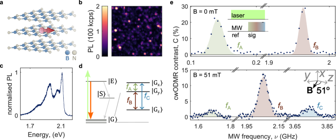
a Schematic of the hBN layers containing a spin defect with in-plane spin principal axis. 3D model of the crystalline structure was generated using ref. 67. b Spatial photoluminescence (PL) map of a hBN device containing individually addressable defect centres. c PL spectrum of the carbon-related defect in hBN. d Schematic of the electronic level structure of the defects, consisting of ground and optically excited-state manifolds, and a metastable state. Relaxation from the optically excited-state to the ground-state manifold can occur radiatively (solid orange arrow) or non-radiatively (dashed grey arrows) through a sequence of direct and reverse intersystem crossing events. The ground-state manifold is a spin-1 with non-degenerate spin sublevels at zero magnetic field. Spin-resonance transitions between each of the three spin sublevels are possible, giving rise to three spin-resonance signatures, labelled fA,B,C in ascending energy. e cwODMR spectra measured at 0 mT (top panel) and 51(1) mT (bottom panel), showing three spin transitions between the spin sublevels of an S = 1 system. Blue circles are measured mean values, with grey error bars indicating the standard error of the mean. Shaded regions are fits to the data using a Gaussian peakshape. The inset in the top panel presents the pulse sequence used for detecting cwODMR, whereas the inset in the bottom panel presents the direction of the magnetic field with respect to the defect’s symmetry axes.
Figure 1e (top panel) shows the room-temperature ODMR spectrum for an hBN defect at 0 mT, where the microwaves were applied in the range 0.01–3 GHz. The inset shows the measurement sequence for detecting the continuous wave (cw) ODMR contrast, defined as the relative change in PL under 532-nm illumination induced by the presence of microwaves (C = (PLsig−PLref)/PLref). For this defect, we observe two ODMR resonances, at 0.140(2) and 1.957(1) GHz, with comparable saturated cwODMR contrast of 22(5)% and 30(2)%, (see Supplementary Note 1 for zero-field contrast statistics for a range of defects)39. We assign the ODMR resonances to the transitions of the S = 1 system based on a Hamiltonian of the type,
$$H={H}_{{{{\rm{ZF}}}}}+{H}_{{{{\rm{ZE}}}}},$$
(1)
$${H}_{{{{\rm{ZF}}}}}=D{S}_{z}^{2}+E({S}_{x}^{2}-{S}_{y}^{2}),$$
(2)
$${H}_{{{{\rm{ZE}}}}}=\frac{{\gamma }_{e}}{2\pi }{{{\bf{B}}}}\cdot {{{\bf{S}}}},$$
(3)
where HZF is the zero-field splitting term, HZE is the Zeeman term, D and E are the zero-field splitting parameters that define the defect’s x, y, z principal axes in units of Hz, S is the S = 1 operator with cartesian components Sx,y,z, γe is the electron gyromagnetic ratio, and B is the applied magnetic field. In the absence of applied magnetic field, we only need to consider the HZF term with eigenenergies 0, D−E, and D + E.
The magnitude of the transverse zero-field splitting ∣E∣, relative to |D|, is a measure of the rhombicity, or low symmetry, of the spin density of the system45. In systems where ∣E∣ is low compared to the linewidth (i.e., for the NV centre in diamond and the \({{V}}_{B}^{-}\) defect in hBN), overlapping resonances are observed at zero field, corresponding to transitions between \(\left\vert {m}_{s}=0\right\rangle\) and the near-degenerate \(\left\vert {m}_{s}=\pm 1\right\rangle\), where ms denotes the spin projection along the defect’s z axis46. In such systems, the spin transitions give partial information about the vector of the external magnetic field—while the projection of the field along the z axis (polar dependence) can be determined, the azimuthal direction cannot. In contrast, in the case of low-symmetry S = 1 systems, where ∣E∣ ≠ 0, three transitions may arise between the three spin sublevels at zero field indicated in Fig. 1c45,47,48,49,50. In this case, the transverse zero-field splitting term \(E({S}_{x}^{2}-{S}_{y}^{2})\) hybridises \(\left\vert {m}_{s}=\pm 1\right\rangle\), relaxing the selection rules for transitions between them48. The zero-field spin eigenstates are then given by \(\left\vert {{{{\rm{G}}}}}_{{{{\rm{z}}}}}\right\rangle=\left\vert {m}_{s}=0\right\rangle\), \({\left\vert {{{\rm{G}}}}\right\rangle }_{{{{\rm{x}}}}}=(\left\vert {m}_{s}=+ 1\right\rangle -\left\vert {m}_{s}=-1\right\rangle )/\sqrt{2}\), and \(\left\vert {{{{\rm{G}}}}}_{{{{\rm{y}}}}}\right\rangle=(\left\vert {m}_{s}=+ 1\right\rangle+\left\vert {m}_{s}=-1\right\rangle )/\sqrt{2}\). We assign the zero-field resonances shown in Fig. 1e (top) to the transition between \({\left\vert {{{\rm{G}}}}_{{{{\rm{x}}}}}\right\rangle }\) and \(\left\vert {{{{\rm{G}}}}}_{{{{\rm{y}}}}}\right\rangle\) (fA), and \(\left\vert {{{{\rm{G}}}}}_{{{{\rm{z}}}}}\right\rangle\) and \(\left\vert {{{{\rm{G}}}}}_{{{{\rm{y}}}}}\right\rangle\) (fB), where ∣D∣ = 2.027 GHz and ∣E∣ = 70 MHz for this defect. Previous work on this defect type has reported the presence of all three transitions, but fA was outside of the studied measurement range at zero field39.
Figure 1e (bottom panel) presents the ODMR spectrum for the same defect under 51-mT magnetic field applied in the plane of the hBN layers. At this field, all three spin transitions are visible in the spectrum, with C(fA) = 1.8(2)%, C(fB) = 12.9(5)%, and C(fC) = 2.7(3)%, where C(fi) is the contrast of the i-th transition. We determine that the field vector is at 51(1)° from the defect z axis, parallel to the yz plane, from field-dependent measurements. This means that the defect’s y and z axes are parallel to the plane of the hBN layers, and the x axis is out of the plane. Despite the high off-axis applied field, we observe that the ODMR resonance is not quenched. This is in contrast to what is seen for the NV centre, where a magnetic field ~10 mT misaligned to the defect’s quantisation axis quenches the ODMR resonances due to degradation of the spin initialisation mechanism17,51.
Photodynamics of the carbon-related hBN spin
For optically active spin defects, the ODMR contrast is dependent on the degree of spin initialisation arising from the optical cycle. To understand the remarkably high ODMR contrast and its retention with off-axis field for the hBN defects, we investigate the optical rates of the system by setting up a series of rate equations describing the transfer of population between the electronic states for the model shown in Fig. 2a, in the absence of a magnetic field. Across the defects we study, we observe the magnitude of the saturated zero-field ODMR contrast across the three spin resonances typically follows: C(fA) = C(fB) > C(fC) with defect-to-defect variation in overall magnitude39 (see Supplementary Fig. 2). This observation is in line with an optical defect that shows variable intersystem crossing (ISC) rates, consistent with the variation we see in bunching timescales in second-order autocorrelation (g(2)(t)) experiments37. The non-equal ODMR contrast of fB and fC indicates strong spin selectivity of the ISC at zero-field, as is observed for other low symmetry S = 1 systems47,48,52. In our kinetic model, we hold \({k}_{{{{{\rm{E}}}}}_{{{{\rm{x}}}}}\to {{{{\rm{S}}}}}_{{{{\rm{0}}}}}}={k}_{{{{{\rm{E}}}}}_{{{{\rm{z}}}}}\to {{{{\rm{S}}}}}_{{{{\rm{0}}}}}}\ne{k}_{{{{{\rm{E}}}}}_{{{{\rm{y}}}}}\to {{{{\rm{S}}}}}_{{{{\rm{0}}}}}}\) and \({k}_{{{{{\rm{S}}}}}_{{{{\rm{0}}}}}\to {{{{\rm{G}}}}}_{{{{\rm{x}}}}}}={k}_{{{{{\rm{S}}}}}_{{{{\rm{0}}}}}\to {{{{\rm{G}}}}}_{{{{\rm{z}}}}}}\ne {k}_{{{{{\rm{S}}}}}_{{{{\rm{0}}}}}\to {{{{\rm{G}}}}}_{{{{\rm{y}}}}}}\) in order to restrict the number of fitting parameters, but note that some defects are best described by \({k}_{{{{{\rm{E}}}}}_{{{{\rm{x}}}}}\to {{{{\rm{S}}}}}_{{{{\rm{0}}}}}}\ne {k}_{{{{{\rm{E}}}}}_{{{{\rm{z}}}}}\to {{{{\rm{S}}}}}_{{{{\rm{0}}}}}}\ne{k}_{{{{{\rm{E}}}}}_{{{{\rm{y}}}}}\to {{{{\rm{S}}}}}_{{{{\rm{0}}}}}}\) (\({k}_{S_{0}\to {{{{\rm{G}}}}}_{{{{\rm{x}}}}}}\ne {k}_{S_{0}\to {{{{\rm{G}}}}}_{{{{\rm{z}}}}}}\ne {k}_{S_{0}\to {{{{\rm{G}}}}}_{{{{\rm{y}}}}}}\)).
Fig. 2: Optical and spin dynamics of carbon-related hBN defects.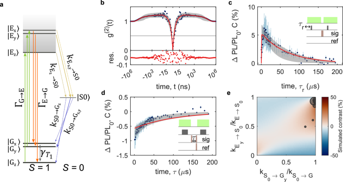
a Model used to fit the results of experiments in (b–d), including a spin-1 ground and optically excited states and a singlet metastable state. Optical excitation and radiative recombination processes are spin-conserving at zero magnetic field. b–d Blue circles correspond to the mean of measured data, light blue error bars indicate one standard deviation of the measured data, red curves correspond to a global fit of the model to the experimental data, and the grey shaded region corresponds to model predictions with b (top) Background-corrected second-order autocorrelation (g(2)(t)). (bottom) Residuals of the fit of the model to the data. c Spin-dependent optical initialisation. Blue circles are the mean value of the contrast measured for various delay times τr. d Modified spin-relaxation experiment. The signal experiment probes the PL when we apply two microwave π pulses, before and after a delay time τ between the two optical pulses. The reference experiment probes the PL when a single microwave π pulse is applied at the end of τ. e Simulated ODMR contrast as a function of the spin-selectivity of the direct (\({k}_{{{{{\rm{E}}}}} \to {{{{\rm{S}}}}}_{{{{\rm{0}}}}}}\)) and reverse (\({k}_{{{{{\rm{S}}}}}_{{{{\rm{0}}}}}\to {{{{\rm{G}}}}}}\)) intersystem crossing rates. The size of the black circles represents cwODMR contrast of different defects, positioned according to their relative rates extracted from fits to second-order autocorrelation and pulsed ODMR experiments. The largest circle corresponds to a 30% contrast.
We estimate the optical rates for a second single defect at zero field via a global fit to the combined results of the second-order autocorrelation (g(2)(t), Fig. 2b), spin initialisation and relaxation measurements (Fig. 2c, d), with the cwODMR magnitude and optical saturation parameters acting as experimental bounds. The pulsed ODMR sequences are illustrated in the insets of the respective figures, where the microwave pulses are π pulses calibrated via Rabi experiments on resonance with fB (see Supplementary Note 3). Figure 2b shows the background-corrected g(2)(t) measurement for this defect (see Supplementary Note 4 for details on the background correction procedure). The horizontal (time) axis is presented in linear scale between −30 and 30 ns, where we can see the characteristic antibunching dip at t = 0. For ∣t∣ >30 ns, we present the time axis in log scale. The hBN defects show significant bunching behaviour, indicative of the presence of a long-lived metastable state, which only subsides after ~100 μs. Similar trends have been reported for various types of hBN emitters37,53,54,55,56,57.
In Fig. 2b–d the red curves are the result of a global fit of a S = 1 optical model to the experimental data, and the grey shaded region reflects the confidence regions for the fits. Table 1 presents the corresponding rates extracted from this fit (see Supplementary Note 5, for details on model, fitting procedure, and uncertainties). We note in our analysis we also considered a model with spin-singlet ground and optically excited states and spin-triplet metastable state, but this model fails to capture the observed behaviour (see Supplementary Note 6). For this defect, the global fit reveals comparable magnitudes for the radiative (ΓE→G = 163 MHz) and non-radiative (\({k}_{{{{{\rm{E}}}}} \to {{{{\rm{S}}}}}_{{{{\rm{0}}}}}}={\sum}_{i={\rm{x,y,z}}} {k}_{{{{{\rm{E}}}}}_{{{i}}}\to {{{{\rm{S}}}}}_{{{{\rm{0}}}}}}=200.8\) MHz) decay rates from the optically excited state, and strongly spin-selective direct and reverse intersystem crossing (\({k}_{ {{{ {\rm{E}} }}}_ {{{ {\rm{y}} }}} \to {{{ {\rm{S}} }}}_ {{{ {\rm{0}} }}} } / {k}_{ {{{ {\rm{E}} }}} \to {{{ {\rm{S}} }}}_ {{{ {\rm{0}} }}} }\) = 0.946 and \({k}_{{{{{\rm{S}}}}}_{{{{\rm{0}}}}}\to {{{{\rm{G}}}}}_{{{{\rm{y}}}}} } /{k}_{{{{{\rm{S}}}}}_{{{{\rm{0}}}}}\to {{{{\rm{G}}}}}}\) = 0.994).
We repeat this procedure for five defects with the same zero-field splitting resonance and find that, while the magnitude of the radiative and intersystem crossing rates are broadly similar across defects, there is significant variation in the ratio of spin-dependent intersystem crossing rates (\({k}_{ {{{ {\rm{E}} }}}_ {{{ {\rm{y}} }}} \to {{{ {\rm{S}} }}}_ {{{ {\rm{0}} }}} } / {k}_{ {{{ {\rm{E}} }}} \to {{{ {\rm{S}} }}}_ {{{ {\rm{0}} }}} }\) = 0.49–0.95, \({k}_{{{{{\rm{S}}}}}_{{{{\rm{0}}}}}\to {{{{\rm{G}}}}}_{{{{\rm{y}}}}}}/{k}_{{{{{\rm{S}}}}}_{{{{\rm{0}}}}}\to {{{{\rm{G}}}}}}\) = 0.82–0.99). This provides an explanation for the defect-to-defect variation (from 39 (see Supplementary Note 7 for extended data from which individual rates are extracted). Figure 2e shows the interdependence of the cwODMR contrast on the spin-selectivity of the direct (\({k}_{{{{{\rm{E}}}}}\to{{{{\rm{S}}}}}_{{{{\rm{0}}}}}}\), vertical axis) and reverse (\({k}_{ {{{ {\rm{S}} }}}_ {{{ {\rm{0}} }}} \to {{{ {\rm{G}} }}} }\), horizontal axis) intersystem crossing rates. The 2D map presents the simulated cwODMR contrast of fB, where the rates indicated in the axes are varied while all remaining rates are kept constant at the values presented in Tab.1. The colour represents the amplitude of cwODMR contrast predicted by the model, with red (blue) regions indicating positive (negative) contrast. The black circles show the experimental cwODMR contrast for each defect we measured (where the size represents the magnitude of cwODMR contrast, see Supplementary Note 8 for the raw spectra), positioned on the map as a function of the determined rates for each defect. The rates extracted using the procedure outlined above for the hBN defects cluster in the top right of the 2D plot, showing that these defects are characterised by strong spin-selectivity in both direct and reverse intersystem crossing processes. The strong spin-dependence of ISC means that spin mixing requires a larger applied magnetic field in order to disrupt the optical spin initialisation mechanism17, giving rise to a large magnetic-field dynamic range for the hBN sensor.
To explore the optical response of the hBN defects to arbitrary oriented applied magnetic field, we perform angular-dependent ODMR (Fig. 3). Figure 3a, c show the dependence of cwODMR central frequencies (top panel) and normalised cwODMR contrast of fA–fC (bottom panels), on the orientation of 51-mT magnetic field in the yz (a) and xy (c) planes, for the same defect that is presented in Fig. 1, where the contrast is normalised by the zero-field cwODMR contrast of fB (experimental data is shown by circles). Interestingly, we see that applied field along the defect y axis (indicated by 90 degrees in Fig. 3a, c) preserves the zero-field contrast. Meanwhile, the cwODMR contrast of fA (fB) is completely (partially) suppressed as the magnetic field is rotated towards the z axis, while the cwODMR contrast of fC increases (Fig. 3a). We note that the sharp dip in contrast of fA and fB when the field is applied directly along the y axis is reproducible, but we have not identified its origin. Rotation of the applied field in the xy plane away from the y axis leads to a slower suppression of the cwODMR contrast of both fA and fB, with a correspondingly slower increase of the cwODMR contrast of fC (Fig. 3c).
Fig. 3: Magnetic-field orientation and amplitude dependence of cwODMR.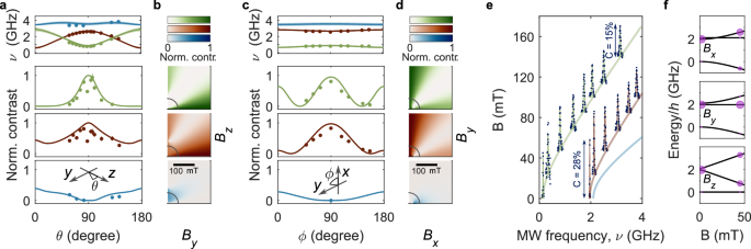
a Angular magnetic-field dependence of cwODMR frequency (top panels) and contrast of resonances fA to fC (top to bottom), normalised by the zero-field cwODMR contrast of the fB resonance, with 50-mT bias magnetic field applied in the yz plane. Data are presented as circles, with colour coding according to the inset of Fig. 1d, and curves indicate the cwODMR contrast simulated using the model of Fig. 2 and fit parameters presented in Tab.1. The inset indicates the direction of rotation of the bias magnetic field. b Calculated contrast of each resonance as a function of By and Bz. c as (a), but with 50-mT bias field applied in the xy plane of the defect (ϕ varies with fixed θ = 85°). d Calculated contrast of each resonance as a function of Bx and By. e Persistence of saturated cwODMR contrast for field applied along the defect y direction (ϕ = 90°, θ = 85°), shown up to 140 mT. The solid curves represent the transition frequencies of fA (green), fB (red), and fC (blue) resonances as a function of By amplitude. The measured cwODMR contrast as a function of MW frequency is represented by blue circles. f Evolution of spin eigenstates of the Hamiltonian Eq. (1) with applied magnetic field along the x, y, z axes of the defect, from top to bottom. Calculated amplitudes of the optically initialised population of each spin sublevel are indicated by the size of the purple circles.
The experimental data in this figure (circles) is shown alongside the results of the modelled cwODMR contrast (solid curves (Fig 3a, c) and 2D colour maps (in Fig 3b, d)) for this defect, determined from the zero-field rates obtained in the analysis above, where we include the effect of magnetic field by introducing the Zeeman term to the spin Hamiltonian (HZE). We determine the magnetic-field-dependent intersystem crossing rates from a statistical average of the zero-field rates, such that \({k}_{ij}({{{\bf{B}}}})={\sum }_{p,q}| {a}_{ip}{| }^{2}| {a}_{jq}{| }^{2}{k}_{pq}^{0}\), similar to the approach taken by Epstein et al. and Tetienne et al. for the NV centre in diamond17,58. Here, \({k}_{pq}^{0}\) are the zero-field direct and reverse spin-dependent intersystem crossing rates; the coefficients aip can be obtained by comparing the zero-field eigenstates (\(\left\vert p(0)\right\rangle\)) to the eigenstates of the Hamiltonian at a field (\(\left\vert i({{{\bf{B}}}})\right\rangle\)), such that \(\left\vert i({{{\bf{B}}}})\right\rangle={\sum }_{p}{a}_{ip}\left\vert p(0)\right\rangle\). In the absence of spectroscopic information about the excited-state zero-field splitting configuration, we assume equal zero-field splitting parameters in ground and optically excited states, and this assumption has no significant implication on the findings of this work (see Supplementary Note 9).
Figure 3b, d shows the calculated normalised contrast of each cwODMR resonance for this defect as a function of By and Bz (Bx) up to 200 mT with Bx (Bz) fixed at 0 mT. These simulations show that the behaviour outlined above persists for a wide range of bias magnetic field values, with limited regions showing complete quenching of all three cwODMR resonances. Figure 3e presents the experimental cwODMR spectra as a function of By amplitude up to 140 mT, showing that for this class of defects, contrast is preserved for an applied field along the defect’s y axis. Importantly, this data reveals a spin system with multiple quantisation axes, where optical initialisation of each spin transition has a different dependency on the orientation of the applied field45.
Figure 3f presents the evolution of the ground-state spin eigenstates for the hBN defect system under applied magnetic field in the x, y, z direction (top to bottom panels). The purple circles represent the simulated optically initialised population, calculated based on the model above and using the representative rates of Tab.1. As observed experimentally, in the zero-field limit, the kinetic model predicts the system is initialised into the \(\left\vert {{{{\rm{G}}}}}_{{{{\rm{y}}}}}\right\rangle\) state, giving rise to strong fA and fB and weak fC (Fig. 1). Magnetic field applied along the defect y axis (middle panel) mixes \({\left\vert {{{\rm{G}}}}_{{{{\rm{x}}}}}\right\rangle }\) and \(\left\vert {{{{\rm{G}}}}}_{{{{\rm{z}}}}}\right\rangle\), preserving the zero-field character of \(\left\vert {{{{\rm{G}}}}}_{{{{\rm{y}}}}}\right\rangle\), thus retaining the zero-field spin initialisation and ODMR contrast. Conversely, applied field along x (z) mixes \(\left\vert {{{{\rm{G}}}}}_{{{{\rm{y}}}}}\right\rangle\) and \(\left\vert {{{{\rm{G}}}}}_{{{{\rm{z}}}}}\right\rangle\) (\({\left\vert {{{\rm{G}}}}_{{{{\rm{x}}}}}\right\rangle }\)), redistributing the zero-field initialised population and modifying the saturated cwODMR contrast of each resonance with respect to their zero-field values. In total, the experimental data and kinetic model both reveal a multi-axis sensor with optical initialisation dynamics that enable operation under strong off-axis field.