Here, we provide additional detail regarding the continuum description of the wave-packet preparation, how to determine clock precision \({{{\mathcal{N}}}}_{\varSigma }\) and \({{{\mathcal{N}}}}_{\infty }\) from the Lindbladian, and how the precision-entropy scaling is derived. Furthermore, details are provided on how to obtain the master equation model of the main text from an extensible microscopic model, and finally, technical aspects regarding the robustness against perturbations are given.
Hydrodynamical continuum limit
In the limit of large values for the number of ring sites n, the wave-packet propagation can be described using a continuum description, where we define the real space coordinates as xj = j/λℓ and go from the discrete coordinates j = 0, 1, …, n − 1 to the continuum \(x\in \left[0,n/{\lambda }_{\ell }\right)\to {{\mathbb{R}}}_{+}\) in the limit n ≫ λℓ. The particle density \(n(t,{x}_{j})={\lambda }_{\ell }^{-1}{| \left\langle j| \psi (t)\right\rangle | }^{2}\) can be described by the evolution equation
$${\partial }_{t}n(t,x)=-2{\partial }_{x}(g(x)n(t,x)),$$
(8)
where g(x) is defined by the coupling constant g(xj) = gj. The equation of motion for n(t, x) follows from the continuum limit of the Schrödinger equation \(i{\partial }_{t}\left\vert \psi (t)\right\rangle =H\left\vert \psi (t)\right\rangle\), and conserves probabilities \(1=\int_{0}^{\infty }{{\rm{d}}}x\,n(t,x)\). The continuum model is valid so long as we consider times t n/(2g) where the wave packet has not yet reached the right ramp of the coupling potential (equation (6)), and furthermore λℓ, n ≫ 1, to ensure that g(x) and n(t, x) do not vary quickly on the lattice length scale. The derivation of the continuum model is discussed in further detail in Supplementary Section C1, where we also provide the analytical solution for n(t, x). The numerics confirm that the continuum limit captures well the scaling behaviour of the discrete wave function beyond the length scale of the lattice. In particular, we find that the initial distribution n(0, x) is transported to x > 0 and broadened by the width λℓ of the initial ramp. This leads to the scaling form \({| \left\langle j| \psi (t)\right\rangle | }^{2} \sim {\lambda }_{\ell }^{-1}f{((j-2gt)/{\lambda }_{\ell })}^{2}\) of the wave packet in the limit of large times and and displacement x, 2gt ≫ λℓ, where f is some function independent of n and λℓ describing the shape of the travelling wave packet.
Clock precision with full counting statistics
The definitions brought forward in equations (4) and (5) of the main text defined clock precision relative to the tick number statistics \({{{\mathcal{N}}}}_{\varSigma }={\lim }_{t\to \infty }{{\rm{E}}}[N(t)]/{{\rm{Var}}}[N(t)]\) and relative to the waiting time statistics \({{{\mathcal{N}}}}_{\infty }={{\rm{E}}}{[T]}^{2}/{{\rm{Var}}}[T\,]\). Here, we provide the necessary details to calculate these two quantities based on the Lindblad master equation \({{\mathcal{L}}}={{{\mathcal{L}}}}_{0}+{{{\mathcal{L}}}}_{+}+{{{\mathcal{L}}}}_{-}\). The decomposition of the Lindbladian into three terms separates out the ‘no jump’ part
$${{{\mathcal{L}}}}_{0}\,\cdot \,=-i[H,\,\cdot \,]-\frac{1}{2}\{\,{J}^{{\dagger} }J,\,\cdot \,\}-\frac{1}{2}\{\,{\overline{J}}^{{\dagger} }\overline{J},\,\cdot \,\},$$
(9)
describing the non-Hermitian evolution conditioned on no jumps. The jumps generated by J defining positive ticks are described by \({{{\mathcal{L}}}}_{+}\,\cdot \,=J\cdot {J}^{{\dagger} }\), and the ones for \(\overline{J}\), the negative ticks, by \({{{\mathcal{L}}}}_{-}\,\cdot \,=\overline{J}\cdot {\overline{J}}^{{\dagger} }\). The late time statistics of N(t) are fully determined by introducing the tilted Liouvillian73
$${{\mathcal{L}}}(\,\chi )={{{\mathcal{L}}}}_{0}+{{\mathrm{e}}}^{i\chi }{{{\mathcal{L}}}}_{+}+{{\mathrm{e}}}^{-i\chi }{{{\mathcal{L}}}}_{-},$$
(10)
with discrete counting field χ. The eigenvalue λ(χ) of \({{\mathcal{L}}}(\,\chi )\) that has the largest real value is equal to the cumulant generating function t−1C(χ, t) of N(t) at late times, and thus, we can determine the kth cumulant
$${\lim }_{t\to \infty }{t}^{-1}\langle \langle N{(t)}^{k}\rangle \rangle ={\left(-i{\partial }_{\chi }\right)}^{k}\lambda (\chi ){| }_{\chi = 0}.$$
(11)
The special cases k = 1, 2 give the expectation value and variance of N(t) needed to determine the clock precision \({{{\mathcal{N}}}}_{\varSigma },\) as further detailed in Supplementary Section D1.
In the limit where \({{{\mathcal{L}}}}_{-}=0\), that is, the limit of infinite entropy production, the counting variable N(t) is a renewal process54, that is, the time between each increment of N(t) is an independent and identical copy of the waiting time T. In this limit, the late time cumulants of N(t) are fully determined by the statistics of T, and one can relate16,54
$${\lim }_{t\to \infty }\frac{{{\rm{E}}}[N(t)]}{t}=\frac{1}{{{\rm{E}}}[T\,]},\quad {\lim }_{t\to \infty }\frac{{{\rm{Var}}}[N(t)]}{t}=\frac{{{\rm{Var}}}[T\,]}{{{\rm{E}}}{[T\,]}^{3}},$$
(12)
showing that \({{{\mathcal{N}}}}_{\varSigma }\to {{{\mathcal{N}}}}_{\infty }\) as Σtick → ∞. The waiting time statistics for \({{{\mathcal{L}}}}_{-}=0\) can also be determined directly with the Liouvillian, \(E[{T}^{k}]\)\(={(-1)}^{k}k!{{\rm{tr}}}[{{{\mathcal{L}}}}_{0}^{\,-k}{\rho }_{0}]\). A detailed derivation can be found in Supplementary Section B1.
As for the introductory statement that \({{{\mathcal{N}}}}_{\infty }\) equals how many times the clock ticks until it misses one tick compared with the perfect parameter time, it can be shown to be consistent with the definition \({{{\mathcal{N}}}}_{\infty }={{\rm{E}}}{[T\,]}^{2}/{{\rm{Var}}}[T\,]\) (ref. 12). As the time between ticks is independently and identically distributed, the variance of the time to the kth tick is given by Var[Tk] = kVar[T]. Setting the standard deviation of the kth tick to equal the time between two ticks \({{\rm{Var}}}{[{T}_{k}]}^{1/2}\equiv {{\rm{E}}}[T\,]\), we can formally solve for k to give \(k={{{\mathcal{N}}}}_{\infty }\), recovering the initial statement.
Theory of the precision–entropy scaling
In case of finite entropy dissipation, the master equation is perturbed by a term describing the negative ticks, which is of magnitude \(\delta ={{\mathrm{e}}}^{-{\varSigma }_{{{\rm{tick}}}}}\). In the limit of small δ, the clock precision can be expanded in powers of this correction, \({{{\mathcal{N}}}}_{\varSigma }={{{\mathcal{N}}}}_{\infty }+O(\delta )\), using the Landau big-O notation35. Because we aim to minimize entropy Σtick, we want to keep δ as large as possible while at the same time making sure the precision \({{{\mathcal{N}}}}_{\varSigma }\) is sufficiently close to \({{{\mathcal{N}}}}_{\infty }\).
If δ = n−ζ decays algebraically for some exponent ζ > 0 large enough to cancel out the constant factors in the big-O correction, the entropy scales only logarithmically while at the same time keeping the perturbations due to the negative ticks small. How large ζ needs to be is determined in part by the spectral gap of the system’s Lindbladian and by whether it scales algebraically with system size (which is related to the famously hard problem of undecidability of the existence of spectral gaps74; Supplementary Section D). We have numerically determined the scaling up to n = 200 and found that the choice ζ = 4 is sufficient to make the error between \({{{\mathcal{N}}}}_{\varSigma }\) and \({{{\mathcal{N}}}}_{\infty }\) arbitrarily small as n grows. Using the identity \(\log \delta =-{\varSigma }_{{{\rm{tick}}}}\), we find the entropy scales logarithmically \({\varSigma }_{{{\rm{tick}}}}=\zeta \log n\), whereas \({{{\mathcal{N}}}}_{\varSigma } \sim {n}^{1.31}\) scales polynomially (with the negligible correction), which results in equation (1).
Applicability of the master equation
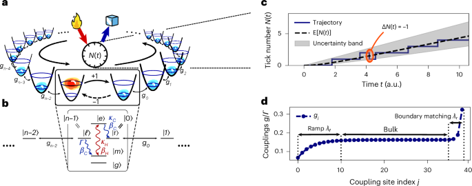
Using spin chains or CCAs to model the ring clock from the main text leads to an effective description with the Hamiltonian H as in equation (2) and jump operators \(J,\overline{J}\). Working with a spin chain, the local Hamiltonians are given by \(\frac{\omega }{2}{\sigma }_{z,\,j}\) for site j, and the nearest-neighbour coupling can be modelled by the particle number conserving hopping term gjσ−,jσ+,j+1 + h.c. The challenging part for a microscopic description comes from the fact that we have to prevent multiple excitations entering the ring at once to ensure that the description we have used so far is valid. One way to solve this problem is to treat the first and the last site of the ring clock separately as a single system—the ticking element—as proposed in Fig. 1b. To ensure that we recover the effective dynamics described in the main text, this ticking element has to (1) remember when it has emitted an excitation into the ring such that it does not emit another excitation into the ring before it has ticked, and (2) it has to be boundary-matched to the ring couplings gj to avoid the reflection of the incoming wave packet.
The proposed level scheme comprises five states and undergoes the following cycle for a tick: \(\left\vert g\right\rangle \to \left\vert \ell \right\rangle \to \left\vert m\right\rangle \to \left\vert e\right\rangle \to \left\vert r\right\rangle \to \left\vert g\right\rangle\). Note, we identify \(\left\vert \ell \right\rangle \equiv \left\vert n-1\right\rangle\) as formally the last ring site in terms of the states of the reduced model, and \(\left\vert r\right\rangle \equiv \left\vert 0\right\rangle\) as the first site. The idea of this scheme is that, by adiabatically eliminating the intermediate states \(\left\vert m\right\rangle\) and \(\left\vert e\right\rangle\) from the tick cycle, we recover the jump process \(\left\vert n-1\right\rangle \equiv \left\vert \ell \right\rangle \to \left\vert 0\right\rangle \equiv \left\vert r\right\rangle\) generated by J (and the inverse generated by \(\overline{J}\)). To get there, we look into each step of the tick cycle separately. When the excitation is in the ring, the ticking element is in the ground state \(\left\vert g\right\rangle\). When the excitation arrives at the site \(\left\vert n-2\right\rangle\) in the ring, it couples to the transition \(\left\vert g\right\rangle \to \left\vert \ell \right\rangle\) with strength gn−2. In turn, the state \(\left\vert \ell \right\rangle\) decays dissipatively as \(\left\vert \ell \right\rangle \to \left\vert n\right\rangle\) with rate Γ, which defines the tick. This is the rate that crucially has to be boundary matched to the couplings gj, and the strength of the reverse process needs to be suppressed with the entropy production Σtick by coupling this transition to a cold enough bath at inverse temperature βC. After this decay, however, the system is not in resonance with the frequency ω of the ring structure anymore and it has to brought to a higher energy again, for which two additional dissipative drives can be used. With an additional hot bath at inverse temperature βH driving \(\left\vert m\right\rangle \leftrightarrow \left\vert e\right\rangle\) at a rate κH and an additional cold bath at inverse temperature βC mediating \(\left\vert e\right\rangle \to \left\vert r\right\rangle\) at a rate κC, we can create a population inversion to ensure that, in the end, the state that arrived on the ring ends up on \(\left\vert r\right\rangle\). Then, the ticking element is again on resonance with ω, and the excitation can be coherently coupled to the next site with strength g0, completing the cycle.
When the excitation is in the ring, the ticking element latches to the ground state \(\left\vert g\right\rangle\), which is not addressed by the thermal drives, and therefore, no second excitation is emitted into the ring. So long as ω ≫ κH, κC, Γ ≳ gj is the hierarchy of energy scales in the problem, the Lindblad master equation is applicable in a local picture with weak interactions despite the many-body nature75,76, and the notion of entropy Σtick we used coincides with the thermodynamic entropy from Clausius’ law77 as in equation (3).
Stability under perturbations
In a realistic experimental implementation of the ring clock, the actual nearest-neighbour couplings would differ slightly from the ideal choice gj. From the disorder in the couplings, we would expect the clock to perform worse due to imperfect preparation of the travelling wave packet in the preparation region, off-diagonal Anderson localization in the bulk78,79,80,81 and reflection in the final region of the ring. Furthermore, in a realistic scenario, the bulk of the ring would not be perfectly isolated from the environment. As a result, the bulk sites may absorb excitations from the environment, or lose them, negatively impacting the precision. We analyse the stability of the main result equation (1) under these two perturbations of the ideal scenario. In a concrete experimental realization, further sources of error may contribute depending on the details of the physical platform, such as disorder in the bare qubit frequencies in superconducting circuits, whose impact we expect to be comparable to that of imperfections in the couplings gj.
For a fixed but small error εloc in the nearest-neighbour couplings or an unwanted coupling εenv to the environment, the predicted precision scaling from equation (7) can be upheld up to some finite ring length \({n}_{\max }\). For longer rings, the errors start to dominate and the precision decreases again (Extended Data Figs. 2a and 3a). The analysis in the following shows that this point of breakdown \({n}_{\max }\) of the optimal scaling increases the smaller the error ε in the couplings and dissipation is with the precise relationship of the form
$${n}_{\max } \sim \frac{1}{{\varepsilon }^{\kappa }},$$
(13)
where κ > 0 is some exponent that depends on the type of error. This relationship (equation (13)) is algebraic rather than exponential, and in the following we determine the exponents κloc for the parameter perturbations as well as κenv for the environmental perturbation seperately.
Disorder in the couplings
The error model for the couplings gj perturbs each nearest-neighbour coupling with a multiplicative factor \({(1+{\varepsilon }_{{{\rm{loc}}}})}^{\hat{{X}}_{j}}\), where ε > 0 is the error and \({\hat{X}}_{j} \sim {{\mathcal{N}}}(0,1)\) is normally distributed with mean 0 and variance 1. To create Extended Data Fig. 2a, for a fixed ring length n and error ε, M = 400 independently and identically distributed (i.i.d.) samples of perturbed couplings \({\tilde{g}}_{j}\) are generated, leading to a perturbed precision value \({\tilde{{{\mathcal{N}}}}}_{\infty }\). Then, a statistical average is taken \({\langle {\tilde{{{\mathcal{N}}}}}_{\infty }\rangle }_{\hat{X}}\) over the M random choices of disordered parameters \({\tilde{g}}_{j}\). It can be seen that, for εloc fixed, this average value increases until a saddle point \({n}_{\max }\) is reached and the precision decreases again. If we fit a linear slope (black dashed line) in the log–log scale through the maxima of the average curves for all error values, we find that the precision still scales as ~n1.39(5), albeit with a constant factor smaller in comparison with the optimal scaling. This scaling approximately agrees with the ideal one. The uncertainty in the exponent comes from the distribution of the numerically determined maxima and is determined with the covariance matrix from the linear regression. Extended Data Fig. 2b shows how this maximal length \({n}_{\max }\) changes as a function of the εloc and a linear fit in the log–log plot reveals a scaling exponent κloc = 0.81(3) for equation (13). The uncertainty in the exponent comes from the statistical distribution of the data points \({n}_{\max }\) and is determined again using the covariance matrix from the linear fit. Note that the maximum ring length in this analysis is of the order n = 300 owing to limitations in the computational runtime for the statistical averaging.
Undesired environment interactions
In the ideal clock model, the ticks are generated by \(J=\sqrt{\varGamma }\left\vert 0\right\rangle \left\langle n-1\right\vert\). To model erroneous losses due to the environment along the ring in the spirit of the abstract model, we assume that these decays are also registered as ticks leading to a premature reinitialization of the clock akin to the tick process defined by the jump operator J. This lowers the expected time between two ticks E[T] and increases the variance Var[T], thus overall decreasing the clock precision \({{{\mathcal{N}}}}_{\infty }\). For an actual experimental realization of the ring clock, this description is of course only an approximation of how losses would impact the result, but it captures the main features of such imperfections. We include these processes with additional dissipators in the master equation description \({L}_{j}=\sqrt{\varGamma {\varepsilon }_{{{\rm{env}}}}}\left\vert 0\right\rangle \left\langle j\right\vert\) for sites j = 1, …, n − 2, where εenv > 0 is the fractional error in the dissipation. For a finite-temperature environment, however, also the reverse process \({L}_{j}^{{\dagger} }\) is possible. Due to detailed balance, the rate of this process is suppressed by a factor \({{\mathrm{e}}}^{-{\varSigma }_{{{\rm{env}}}}}\), where Σenv is the entropy production in the (finite temperature) environment. More importantly, it may also happen that the bulk absorbs a second excitation from the environment, leading to two excitations in the spin chain. If the ring is initially occupied only on site j = 0, …, n − 1, an absorption on any other site i ≠ j can be modelled by the jump operator
$${L}_{(ji),\,j}={{\mathrm{e}}}^{-{\varSigma }_{{{\rm{env}}}}/2}\sqrt{\varGamma {\varepsilon }_{{{\rm{env}}}}}\left\vert\,j,i\right\rangle \left\langle j\right\vert ,$$
(14)
where \(\left\vert\,j,i\right\rangle\) is the state with exactly two excitations, one on each site i and j. Detailed balance guarantees the existence of the reverse process in which the doubly occupied state \(\left\vert\,j,i\right\rangle\) loses an excitation into the environment. This excitation can be lost on both sites i and j. For example, if site i decays, the jump operator is given by \({L}_{j,(ji)}=\sqrt{\varGamma {\varepsilon }_{{{\rm{env}}}}}\left\vert\,j\right\rangle \left\langle j,i\right\vert\). Although, in principle, higher excitation numbers >2 in the ring would be possible, a sufficiently cold environment exponentially suppresses the thermal occupation probability of these higher subspaces. In this context, already a logarithmically growing inverse temperature \({\beta }_{{{\rm{env}}}} \sim \log n\) of the environment is sufficient. At the same time, an environment temperature with such scaling ensures that the entropy produced by an excitation \({\varSigma }_{{{\rm{env}}}}={\beta }_{{{\rm{env}}}}\omega \sim \log n\) grows logarithmically only in the ring length (for fixed bare spin frequency ω). An exact and effective treatment of the single- and double-excitation subspaces thus captures the dominant error contributions to the clock precision (see details in Supplementary Section E).
In Extended Data Fig. 3a, we show how the precision \({{{\mathcal{N}}}}_{\varSigma }\) scales as a function of the ring length, n, for a selection of fixed errors εenv, and with entropy \({\varSigma }_{{{\rm{env}}}}=\frac{3}{2}{\varSigma }_{{{\rm{tick}}}}\) also only logarithmically growing with chain length. For up to n = 12 sites, we numerically simulate the full dynamics in the double-excitation subspace, while for 12 ≤ n ≤ 200 we use a computationally efficient, effective model for extrapolation (see details in Supplementary Section E). The inset in Extended Data Fig. 3a shows that the difference between exact and effective model vanishes for growing n, supporting the applicability of the effective model. Similar to the coupling perturbations we find that, for every fixed error εenv, there is a turn-around point \({n}_{\max }\), where the precision reaches its maximum and after which the precision decreases as the ring gets longer. A fit (dashed black line) through all the maxima recovers a polynomial scaling of the precision, ~n1.23(1). Together with \({\varSigma }_{{{\rm{env}}}} \sim \log n\), this still guarantees an exponential precision–entropy relationship, albeit with a lower exponent than in the idealized case. We show the log–log relationship between εenv and \({n}_{\max }\) in Extended Data Fig. 3b, where a linear fit reveals a an exponent κenv = 0.43 following equation (13). We further observe that the ring clock is more sensitive to amplitude damping noise in the bulk than to disorder in the couplings, as the tolerable loss εenv is smaller than the coupling error εloc; yet, in both cases, the scaling with \({n}_{\max }\) remains algebraic.