Simulations
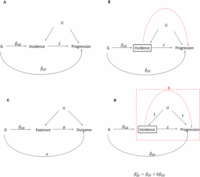
In order to test this novel application of the method we first simulated GWAS of disease incidence and progression, using knowledge of chronic kidney disease to approximately inform modelling choices. Genotypes were simulated for 10,000 individuals at 2000 independent SNPs in Hardy-Weinberg equilibrium [14] and in linkage equilibrium. 95% of SNPs had no effect on disease incidence or progression (G0), 1% of SNPs had effects on disease incidence only (GI), 1% of SNPs had effects on disease progression only (GP) and 3% of SNPs had effects on both incidence and progression (GIP), with correlated \({\beta }_{G{X}_{i}}\) and \({\beta }_{G{Y}_{i}}\) with correlation coefficient ρ (constant across GIP variants). This set-up produces a large pleiotropic cluster of variants explaining more of the phenotypic variance of disease progression than the non-pleiotropic cluster. This situation is likely to violate the assumptions of both the Dudbridge and Slope-Hunter methods, but is a plausible architecture of chronic kidney disease related traits. In order to approximate realistic distributions of effect sizes across the range of allele frequencies, minor allele frequencies were first drawn from a uniform distribution between 0.01 and 0.49, and standardised effect sizes were defined as \(\pm \surd \frac{{r}^{2}}{2{maf}\left(1-{maf}\right)}\) where variant level r2 values were drawn from the positive half of a normal distribution with mean 0 and standard deviation \(\frac{R^2\sqrt{\pi}}{n\sqrt{2}}\), where \(R^2\) is the phenotypic variance explained by the cluster and n is the number of SNPs in the cluster. Confounders U were simulated as a random normal variable, and disease incidence (Inc) was initially simulated under a liability threshold model where the liability had a 40% SNP heritability according to the equation:
$${In}{c}_{j}={\sum}_{i=1}^{2000}{\beta }_{G{X}_{i}}{G}_{{ij}}+{U}_{j}+{\epsilon }_{{I}_{j}}$$
A threshold value of the Inc phenotype was selected to define the binary phenotype of incident CKD such that the prevalence of CKD in the simulated population was 40%. Kidney function decline or disease progression was then simulated in all participants as a continuous variable with genetic effects on progression scaled such that the phenotype has 30–40% SNP heritability (estimated in GWAS among the entire simulated population) and 30–40% of its variance explained by the confounders U, according to the equation
$${Pro}{g}_{j}={\sum}_{i=1}^{2000}{\beta }_{G{Y}_{i}}{G}_{{ij}}+\lambda {In}{c}_{j}+\gamma {U}_{j}+{\epsilon }_{{P}_{j}}$$
The values of λ and γ (Fig. 1) were set as 0.1 and 1.5 respectively for all simulations. GWAS of the binary CKD incidence phenotype was then performed in the whole population (logistic regression), and GWAS of the CKD progression phenotype was performed in only those simulated participants with incident CKD. Simulations were repeated with differing values of ρ.
We then applied Dudbridge’s method, the Slope-Hunter method, and the MR-Horse method to these GWAS results. For both Dudbridge and Slope-Hunter methods, only variants associated with disease incidence (we employed a threshold of p b. The Hedges-Olkin approximation was used to adjust Dudbridge estimates for measurement error, as the alternative simulation extrapolation methods performed unpredictably at extremes of genetic correlation. Confidence intervals for the Slope Hunter estimates were bootstrapped over 200 iterations. The prior probabilities for the MR-Horse model parameters were informed by knowledge of chronic kidney disease. The prior probability for ρ was \(2r{{{\mbox{-}}}}1\) where \(r\sim {Beta}\left(3,1\right)\). This prior puts most of the probability weighting around high positive correlation but allows for some lower and even negative correlation for some variants. The prior probability distribution for the global shrinkage parameter τ was set as \(\tau \sim {Cauch}{y}^{+}\left(0,1\right)\), and the prior for the local shrinkage prior \({\phi }_{i}\) was \({\phi }_{i}\sim {Cauch}{y}^{+}\left(0,1\right)\). Uninformative priors were used for \(b\sim {Uniform}\left(-10,10\right)\), \(\mu \sim N\left(0,1\right)\) and \({s}_{x}^{2}\sim {N}^{+}\left(0,1\right)\). Posterior parameter estimates were drawn from four parallel Markov Chains simulated in JAGS using 15,000 iterations with a 20% burn-in. Power, type 1 error and bias were recorded across 1000 simulation iterations. For better comparison of method performance, power was measured across the entire range of simulated variant effect sizes. Type 1 error was defined as the identification of a significant association of a GI or G0 SNP with disease progression. Significant effects were defined at p \({\beta }_{G{Y}_{i}}\) did not include 0. Bias was defined as \(|{\hat{\beta }}_{G{Y}_{i}}-{\beta }_{G{Y}_{i}}|\) for each method.
Sensitivity analyses were performed including simulated populations of different sizes, different relative cluster sizes (testing relative performances of the adjustment methods when assumptions of the other methods are met), and sparser or less sparse MR-Horse prior distributions for \({\beta }_{G{Y}_{i}}\) (Supplementary Data).
All analyses were performed in R 4.3.1 and JAGS 4.3.2 on the Oxford University Medical Sciences Division Biomedical Research Computing Cluster.
Application to CKDGen data
To illustrate the performance of our method in a real dataset we used data from large meta-analyses of GWAS of kidney disease traits performed by the CKDGen consortium. We used summary statistics from two GWAS: (i) a GWAS of creatinine-based eGFR from Wuttke et al. [15] and (ii) a GWAS of eGFR decline over time, adjusted for baseline eGFR from Gorski et al. [13]. As pointed out by the authors, adjustment for eGFR in GWAS (ii) should introduce a collider bias effect and spurious associations between genetic variants associated with cross-sectional eGFR alone and eGFR decline. Notably this scenario of adjustment for a baseline variable is different to our simulated scenario of stratification by incident disease, but the use of creatinine-based eGFR measurements as the phenotype of interest has the illustrative advantage that genetic variants with a known functional role in creatinine production (or associated only with creatinine-based measurements of kidney function and not with cystatin-c or urea-based measurements) are unlikely to have true causal associations with kidney function decline over time. Associations with such variants in GWAS (ii) at the GATM, CPS1, and SHROOM3 loci are likely to be due to bias and should be attenuated by an adjustment method which successfully reduces collider bias. They therefore can be used as a form of negative control. Conversely, associations with genetic variants at loci with probable true effects on kidney function decline over time (associated with multiple measures of kidney function or known implication of nearby genes in Mendelian kidney disease) should be relatively preserved.
We identified a set of independent genetic variants in the Gorski et al. summary statistics using the PLINK 1.9 “clump” algorithm [16], using the p-value of cross-sectional eGFR associations from GWAS (i) as the clumping parameter with a clumping window of 100 kilobases and an r2 threshold of 0.001.
The MR-Horse model was specified with the same structure and prior probability distributions as above (ie prior probability for ρ placing most probability mass around a correlation between cross-sectional eGFR lowering effects, and faster eGFR decline), and posterior parameter estimates were drawn from four parallel Markov chains with 15,000 iterations and a burn in of 20%. In order to account for the fact that variants were selected for cross-sectional eGFR associations, and that the majority of such variants may have true associations with kidney function decline rendering a sparse horseshoe prior inappropriate, we performed a sensitivity analysis with less and more sparse prior probability distributions for βGY (Supplementary Data). Given that the true genetic architecture of many disease traits of interest is often unknown, sensitivity analyses were also performed using larger and smaller clumping windows for variant selection, and using deliberately mis-specified prior distributions for ρ (Supplementary Data).