Information theory and thermodynamics constitute foundational pillars of modern technology and underpin our understanding of computers and heat engines, respectively. Although these disciplines may seem distinct, they are intricately connected. This connection is encapsulated in Landauer’s principle, first articulated in 19611. Landauer understood that erasing a bit of information in a computer is not for free but is, instead, accompanied by a minimal energy cost dissipated to the environment. Subsequently, various experimental studies2,3,4 have confirmed this lower bound on energy dissipation for near-reversible bit erasure. Logical operations thus imply irreversibility, which poses a fundamental theoretical limitation on the design of any small-scale energy-efficient information-processing technologies5.
However, by extending beyond the case of bit erasure, recent influential work6 has generalized the link between information theory and thermodynamics. Using a quantum statistical mechanics framework, that work reinterprets Landauer’s principle as a means of relating the entropy change of a system to the energy dissipated to its environment in general out-of-equilibrium processes, not just erasure. This relation can be quantified by a measure of process irreversibility7. Such a broader formulation of Landauer’s principle not only deepens its physical importance but also makes this extension particularly relevant for quantum many-body systems, where contributions to irreversibility remain an area of active research, notably for phenomena such as equilibration and thermalization8,9,10,11.
In this work, we employ Landauer’s principle to experimentally characterize the irreversibility of an out-of-equilibrium process in the quantum many-body regime by tracking the time evolution of quantum information-theoretic measures. We present a crisp information-inspired interpretation of the correlations present in states of quantum many-body systems in terms of entropic expressions.
Concretely, we consider a system–environment composite initially in the state ϱSE(0) and evolving under a global unitary time evolution U to the state ϱSE(t) = UϱSE(0)U†. The reduced state of the system S (environment E) is ϱS(E)(t) = TrE(S)[ϱSE(t)], where TrE(S) is the partial trace over the environment (system).
First, let us assume that there are no initial correlations between the system and environment and that the environment is in a thermal state \({\gamma }_{{{\rm{E}}}}^{\;{\beta }_{{{\rm{E}}}}}=\operatorname{e}^{-{\beta }_{{{\rm{E}}}}{H}_{{{\rm{E}}}}}/{{\rm{Tr}}}[\operatorname{e}^{-{\beta }_{{{\rm{E}}}}{H}_{{{\rm{E}}}}}]\) at inverse temperature βE with respect to its Hamiltonian HE. In this case, the entropy production Σ(t), which is a measure of irreversibility6,7,12, can be decomposed as
$$\varSigma (t):= {I}_{{{\rm{SE}}}}(t)+D({\varrho }_{{{\rm{E}}}}(t)\| {\gamma }_{{{\rm{E}}}}^{\;{\beta }_{{{\rm{E}}}}}).$$
(1)
Here, the quantum relative entropy
$$D({\varrho }_{{{\rm{E}}}}(t)\|{\gamma }_{{{\rm{E}}}}^{\;{\beta }_{{{\rm{E}}}}})={{\rm{Tr}}}[{\varrho }_{{{\rm{E}}}}(t)\log {\varrho }_{{{\rm{E}}}}(t)]-{{\rm{Tr}}}[{\varrho }_{{{\rm{E}}}}(t)\log {\gamma }_{{{\rm{E}}}}^{\;{\beta }_{{{\rm{E}}}}}]$$
(2)
quantifies the deviation of the environment from its initial thermal state. The quantum mutual information
$${I}_{{{\rm{SE}}}}(t)=S({\varrho }_{{{\rm{S}}}}(t))+S({\varrho }_{{{\rm{E}}}}(t))-S({\varrho }_{{{\rm{SE}}}}(t))$$
(3)
measures the system–environment correlations, where
$$S(\varrho )=-{{\rm{Tr}}}[\varrho \log \varrho ]$$
(4)
denotes the von Neumann entropy of a state ϱ.
Now we move on to a more general scenario in which the system and the environment are initially correlated, and the state of the environment deviates from thermal equilibrium. We thereby introduce the generalized entropy production ΔΣ ≔ Σ(t) − Σ(0), where the initial correlations and deviations from thermal equilibrium are accounted for by a resource cost \(\varSigma (0)={I}_{{{\rm{SE}}}}(0)+D({\varrho }_{{{\rm{E}}}}(0) \|{\gamma }_{{{\rm{E}}}}^{{\beta }_{{{\rm{E}}}}})\) (ref. 13), with βE being the effective inverse temperature14,15. Landauer’s principle can then be expressed13 as an equality:
$$\Delta \varSigma ={\beta }_{{{\rm{E}}}}\Delta {E}_{{{\rm{E}}}}+\Delta S=\Delta I+\Delta D,$$
(5)
which relates the entropy change of the system ΔS ≔ S(ϱS(t)) − S(ϱS(0)) to the energy dissipated to the environment ΔEE: = Tr[(ϱE(t) − ϱE(0))HE]. In this general formulation, depending on the initial state, ΔΣ is not necessarily non-negative16,17. Alternatively, ΔΣ also decomposes into the change of quantum mutual information ΔI = ISE(t) − ISE(0), which expresses how much the system–environment correlations change along the out-of-equilibrium process, as well as the term \(\Delta D=D({\varrho }_{{{\rm{E}}}}(t)\|{\gamma }_{{{\rm{E}}}}^{\;{\beta }_{{{\rm{E}}}}})-D({\varrho }_{{{\rm{E}}}}(0)\|{\gamma }_{{{\rm{E}}}}^{\;{\beta }_{{{\rm{E}}}}})\), which quantifies how much both the initial state and the final state of the environment are different from the reference equilibrium thermal state. We provide a more thorough motivation for the generalized entropy production ΔΣ in Methods.
Expressed in this form, Landauer’s principle serves as a means of tracking changes in information-theoretic quantities, which compose generalized entropy production ΔΣ in two different ways with a single equation. Herein lies the power at the heart of thermodynamics: just as knowing the precise microscopic degrees of freedom, such as the position and momentum of each particle in a classical gas, is not useful for drawing meaningful conclusions about its dynamics, knowing the density matrix of a quantum many-body system is, similarly, not descriptive. In traditional thermodynamics, the relevant quantities that effectively characterize the dynamics are macroscopic variables like changes in pressure or volume. Similarly, for the out-of-equilibrium dynamics of a quantum many-body system, analysing the information-theoretic quantities in Landauer’s principle allows a simple characterization of its irreversibility.
So far, no systematic experimental pursuit has probed Landauer’s principle in the quantum many-body regime. Here, we address this gap by measuring the time evolution of the different terms in equation (5) in a (1 + 1)-dimensional quantum field simulator of tunnelling-coupled ultracold Bose gases. This experimental platform has proven to be a suitable test bed for simulating one-dimensional quantum field theories. Previous studies using this set-up have examined the area law of quantum mutual information in thermal equilibrium18 and the propagation of second-19 or higher-order correlations20.
In this experiment, two parallel ultracold clouds of 87Rb atoms (Fig. 1a) were confined in highly anisotropic magnetic traps produced by an atom chip21. The clouds were confined in the axial direction (z) by a parabolic trap superimposed with an optical dipole potential to produce hard walls. In the radial directions (x, y), they were confined by a double-well trap with an adjustable barrier between, created by radio-frequency dressing22. The single-particle tunnelling rate can be modified by the amplitude of a radio-frequency field created by two parallel wires on the atom chip.
Fig. 1: Schematic of the experimental protocol.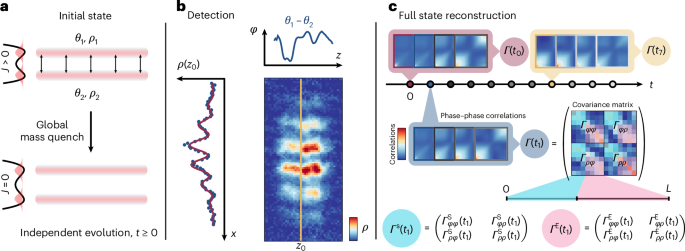
a, The experimental system consists of two tunnelling-coupled ultracold 87Rb gases, with a single-particle tunnelling rate J, initially prepared in an initial state described by a global thermal state of the massive Klein–Gordon Hamiltonian. By ramping up a barrier between the condensates, a global mass quench is performed, and the condensates evolve independently under the post-quench massless Klein–Gordon Hamiltonian for t ≥ 0. b, The atomic clouds are released, and they interfere as they expand. For each experimental realization, we obtained the integrated two-dimensional atomic density with absorption imaging, from which the relative phase profiles were obtained. An example of a fitted phase profile is given for a slice z=z0. c, Using the measured phase–phase correlations, we dynamically reconstructed the covariance matrix for both quadratures. By successively shifting the observation window, we fitted the covariance matrix Γ(t) for different times t. The covariance matrices for the system S and environment E were defined accordingly and used to calculate information-theoretic quantities.
The bosonic quantum field operator for each condensate can be written using the phase–density representation as \({\psi }_{n}(z)=\sqrt{{\rho }_{n}(z)}\operatorname{e}^{\mathrm{i}{\theta }_{n}(z)}\), where θn and ρn denote the phase and density of the respective condensate indexed by n = 1 or 2. In the following, we focus on the operators φ(z) = θ1(z) − θ2(z) and δρ(z) = [ρ1(z) − ρ2(z)]/2, which represent the relative phase and relative density, respectively. These relative degrees of freedom satisfy a similar commutation relation as the original phase and density operators of each condensate, given by [ϕ(z), δρ(z’)] = iδ(z − z’). For strong tunnelling-coupling between the two clouds, the relative degrees of freedom are described by a massive Klein–Gordon Hamiltonian:
$${H}_{{{\rm{KG}}}}=\int_{0}^{L}\,\mathrm{d}z\left[{g}_{{{\rm{1D}}}}\updelta {\rho }^{2}(z)+\frac{{\hslash }^{2}{n}_{{{\rm{1D}}}}}{4m}{({\partial }_{z}\varphi (z))}^{2}+\hslash J{n}_{{{\rm{1D}}}}{\varphi }^{2}(z)\right],$$
(6)
which models low-energy phononic excitations and is an approximation to an interacting sine-Gordon Hamiltonian23 (see equation (11) and below for further details). In equation (6), ℏ is the reduced Planck constant, m is the atomic mass, g1D is the effective one-dimensional atomic interaction strength, L = 49 μm is the axial length of the condensates, n1D ≈ 70 μm−1 is the average linear density and J ≈ 2π × 0.8 Hz is the tunnelling rate introduced before. Note that a mass term appears only due to the tunnelling-coupling between the pair of condensates. A single condensate can simulate only a massless Tomonaga–Luttinger liquid model24,25 (HKG with J = 0).
In our experiments, we prepared the Bose–Einstein condensates in a global thermal state HKG with finite tunnelling-coupling (J > 0). Because we wanted to measure the out-of-equilibrium evolution of information-theoretic quantities, we drove the system out of equilibrium by rapidly quenching J to zero (Fig. 1a). We did so by ramping up the barrier between the condensates within approximately 2 ms. This change corresponds to a global mass quench of the Klein–Gordon Hamiltonian. The condensates then evolved independently under the post-quench massless Klein–Gordon Hamiltonian for times t up to 65 ms.
At each time step t, we turned off all the traps and let the atoms fall freely for 15.6 ms. The clouds then expanded and interfered, resulting in absorption pictures like the one shown in Fig. 1b, which allowed us to measure the spatially resolved relative phase φ(z) between them. Because the detection process is destructive, the measurements were repeated to gather statistics. In our current experimental set-up, the relative density fluctuations δρ were not directly measurable, which prompted the development of a dynamical tomographic reconstruction technique18,26 to access all the elements of the covariance matrix:
$$\varGamma (t)=\left(\begin{array}{cc}{\varGamma }_{\varphi \varphi }(t)&{\varGamma }_{\varphi \rho }(t)\\ {\varGamma }_{\rho \varphi }(t)&{\varGamma }_{\rho \rho }(t)\end{array}\right).$$
(7)
Here, the elements are defined as [Γϕϕ(t)]m,n = 〈ϕ(zm, t)ϕ(zn, t)〉, [Γρρ(t)]m,n = 〈δρ(zm,t)δρ(zn, t)〉 and [Γϕρ(t)]m,n = [Γρϕ(t)]m,nT = 〈(1/2){ϕ(zm, t), δρ(zn, t)}〉, all on a discrete grid with N pixels (m, n ∈ {1, …, N}), which were determined by the resolution constraints of our imaging system, which, thus, introduced an ultraviolet cutoff.
The phase–phase correlations for different evolution times after the quench were measured directly from the extracted relative phase profiles. Assuming that the short-time dynamics after the quench are governed by the massless Klein–Gordon Hamiltonian, then as time progressed, the initial eigenmodes of the relative density transformed into the phase quadrature, and the phase quadrature transformed into the relative density. This transformation allowed us to extract information about these eigenmodes by fitting the initial second-order correlation functions for phase–density and density–density with the observed evolution of the phase–phase correlations in momentum space.
The schematics in Fig. 1c illustrate our dynamical tomographic reconstruction scheme. We followed the technique in ref. 18 for various input intervals with varying starting points. By scanning the starting points of these input intervals throughout the trapping times, we reconstructed the full covariance matrix at every time t, as depicted in Fig. 1. The interval length (32.5 ms, which is close to L/c ≈ 27 ms, where c is the speed of sound) was selected as it was sufficiently long for the slowest eigenmode to acquire enough dynamical phase for a stable reconstruction, yet short enough to prevent mode interactions from affecting the reconstruction. A detailed overview of this reconstruction process is provided in Methods.
The quadratic form of the pre- and post-quench Hamiltonians allowed us to work within the framework of Gaussian quantum information theory27,28. In this framework, the covariance matrix Γ captured all the accessible information about the state of the composite system during the dynamics, from which we extracted all the information-theoretic quantities of interest in equation (5). As has been demonstrated in various experiments23,29,30,31,32, the quadratic approximation of the Hamiltonian accurately captures the dynamics for the timescales considered. Even if the true dynamics deviates from the Gaussian regime and violates the massless Klein–Gordon theory, a Gaussian extremality argument presented in Supplementary Information Section 4 justifies the Gaussian tomography scheme and provides bounds on the information-theoretic quantities. Thus, based on our dynamical tomographic reconstruction of the covariance matrices, Landauer’s principle can also be meaningfully experimentally investigated for interacting models.
Having experimentally reconstructed the post-quench time evolution of the covariance matrices, we partitioned the one-dimensional field of length L into two distinct subregions and split the covariance matrix accordingly (Fig. 1c). Because the quantum field was isolated from its surroundings, one subregion served as the system S with length LS, while the other subregion functioned as the environment E with length LE = L − LS. We probed Landauer’s principle (equation (5)) for various system–environment bipartitions by characterizing the generalized entropy production ΔΣ. To do so, we computed the individual contributions βEΔEE, ΔS, ΔI and ΔD.
The results are presented in Fig. 2 as a function of time for different subregion size ratios and in Fig. 3 as a function of subregion size for different times. The timescales are shown in units of ct/L, where \(c=\sqrt{{g}_{{{\rm{1D}}}}{n}_{{{\rm{1D}}}}/m}\approx 1.8\,\upmu\mbox{m}\,\mbox{ms}^{-1}\) is the speed of sound. Overall, a very good fit of the data (circles) was obtained compared to the theoretical calculations (shaded areas), which used the lowest N = 7 modes, considering the imaging resolution of the experiment. The low-lying modes already capture the dynamics of the continuum theory very well. The error bars representing the 68% confidence intervals were obtained from bootstrapping33 with 999 samples and consider the uncertainty in the tunnelling rate and the estimated initial global temperature. The effective inverse temperature of the environment βE with respect to the post-quench massless Klein–Gordon Hamiltonian was computed using quantum field-theoretic simulations by constructing a global thermal state of the pre-quench massive Klein–Gordon Hamiltonian with the initial global temperature estimated from the experimental data.
Fig. 2: Time evolution of different quantities involved in Landauer’s principle.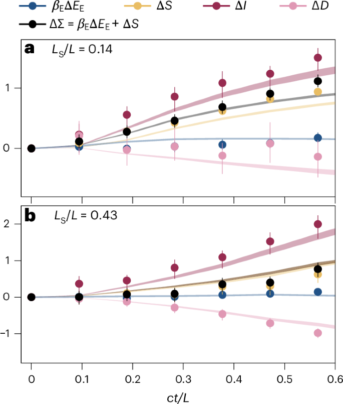
a,b, Quantities of Landauer’s principle are shown as a function of time for subregion size ratios LS/L = 0.14 (a) and LS/L = 0.43 (b). The legend on the top applies to both panels. For each quantity, the experimental averages are represented by circles with error bars marking the 68% confidence intervals (equivalent to the standard error of the mean) obtained from bootstrapping with 999 samples. The shaded areas show the 68% confidence interval for the theoretical predictions, considering the uncertainty in the estimated temperature and tunnelling rate obtained from bootstrapping with 999 samples. The experimental data agree with the quantum field theory simulation results using Neumann boundary conditions and considering the finite imaging resolution.
Fig. 3: Scaling of different quantities involved in Landauer’s principle.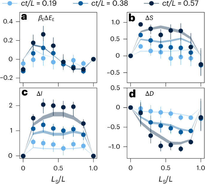
a–d, Quantities involved in Landauer’s principle: βEΔEE, (a), ΔS (b), ΔI (c) and ΔD (d), shown as a function of subregion size for various times ct/L = 0.19, 0.38 and 0.57, as indicated in the legend on top by different colours. The circles represent experimental averages. See Fig. 2 for details of the error bars and shaded areas. The experimental data agree with the quantum field theory simulation results using Neumann boundary conditions.
First, we examine the decomposition of the generalized entropy production ΔΣ into βEΔEE and ΔS. The term associated with the energy dissipated to the environment, βEΔEE, revealed that a small amount of energy flowed into (or out of) the environment for small (or large) systems around ct/LS = 1. However, this term contributed only minimally to the irreversible post-quench dynamics of the quantum field. By contrast, the entropy change of the system, ΔS, dominated the dynamics and showed a clear linear increase up to ct/LS = 1, followed by more pronounced growth. Notably, in Fig. 2, we present only ΔΣ defined by this first decomposition. However, we also found good agreement with the second decomposition (Supplementary Fig. 2), thus providing evidence that the assumptions underlying Landauer’s principle were well satisfied in our experiment.
In comparison to the first, the second decomposition involving ΔI and ΔD shed a slightly different focus on the out-of-equilibrium dynamics. The largest contribution to ΔΣ, the change in quantum mutual information, ΔI, exhibited similar behaviour to ΔS but with a higher magnitude. This increased magnitude was accounted for by the additional entropy change in the environment. However, ΔI competed with the term proportional to the change of the environment, ΔD, which accounted for both the entropic and energetic changes to the environment. This made ΔD a particularly interesting quantity for characterizing the out-of-equilibrium dynamics of the environment experimentally. In our case, ΔD decreased, otherwise mirroring the behaviour of ΔS, due to the small energetic contribution.
To interpret the results, we needed to consider the effects of Neumann and Dirichlet boundary conditions on the quantum field, as shown for the quantum field-theoretic simulations in Fig. 4. These boundary conditions can be contrasted with the curved backgrounds that gave rise to the effective boundary conditions discussed in refs. 19,34. The experimental system exhibited Neumann boundary conditions (∂zφ(z)∣z=0,L = 0) due to the vanishing particle current at the edges. Plots contrasting the scaling with subregion size are shown in Supplementary Fig. 4.
Fig. 4: Quasiparticle interpretation based on quantum field theory simulations.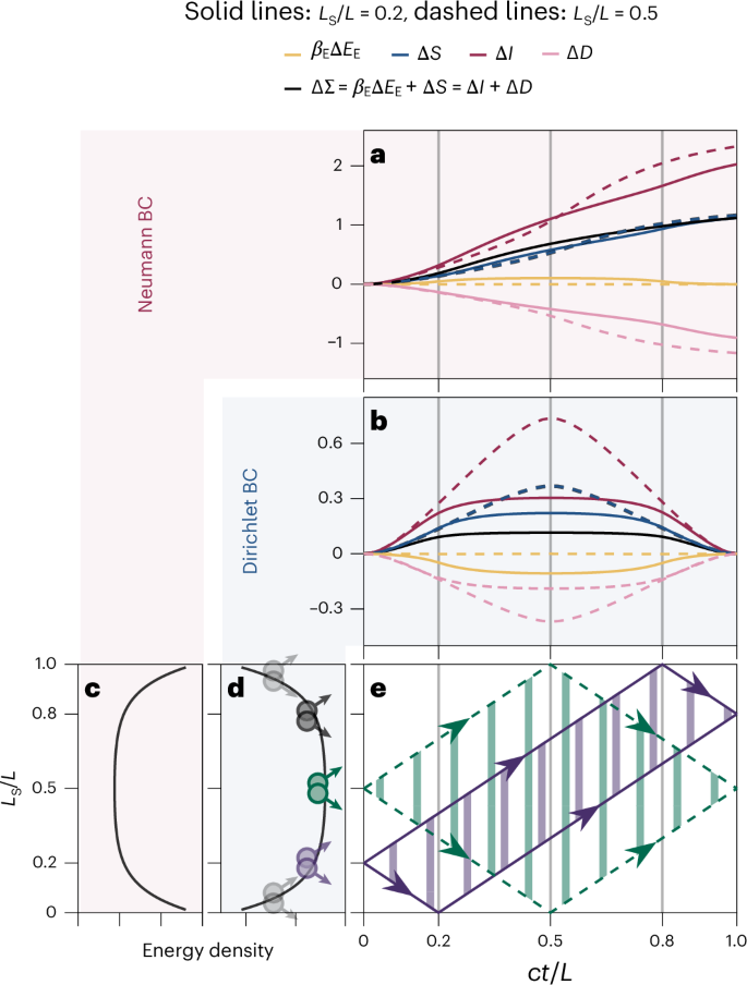
a,b, Time evolution of the quantities involved in Landauer’s principle shown for Neumann boundary conditions (as relevant in the experiment) (a) and Dirichlet boundary conditions (b), using quantum field-theoretic simulations. We interpreted the post-quench dynamics of the global mass quench using a semi-classical quasiparticle picture, as discussed in the text. c,d, Energy density for Neumann boundary conditions (c) and Dirichlet boundary conditions (d). The energetic dynamics can be explained by the difference in the energy density of the initial state at the edges compared to that in the bulk. e, The linear increase in correlations for ct/LS ct/LE > 1, can be explained by the linear effective light cone originating at the system–environment boundary. The effect of the zero mode, present for Neumann boundary conditions, was not captured by the quasiparticle picture for ct/LS > 1. BC, boundary conditions.
However, we first consider simulations with Dirichlet boundary conditions (φ(z)∣z=0,L = 0), which are simpler to understand. Here, the well-established semi-classical quasiparticle picture35 offers a clear and intuitive model for the post-quench dynamics of global mass quenches36,37. The propagation of short-range initial correlations is depicted as occurring through ballistically moving quasiparticles. Following the homogeneous global quench, the initial massive Klein–Gordon thermal state becomes a non-equilibrium state with excess energy relative to the post-quench massless Klein–Gordon Hamiltonian, which governs the time evolution. This initial state acts as a source of quasiparticle pairs emitted globally from every point across the length of the composite system. Each pair in the bulk consists of two quasiparticles correlated with each other and moving in opposite directions at the same speed. For our set of parameters, due to the finite initial correlation length, there exists a small, localized region where quasiparticles are correlated.
In this quasiparticle picture, the change of quantum mutual information ΔI between the system and environment is proportional to the number of pairs of quasiparticles that are shared between the two different subregions. The spread of correlations of short-range interacting models is described by a linear effective light cone originating at the system–environment boundary. The increase in correlations is, thus, proportional to the section of the light cone, or in other words, it is proportional to the distance between the quasiparticles of the pair emitted at the system–environment boundary (Fig. 4e). If the system is smaller than the environment, once the first quasiparticle of this boundary pair reaches the edge of the system at ct/LS = 1 and is reflected, the section of the system–environment boundary pair light cone remains constant. The behaviour of ΔI transitions to a plateau value. From a system perspective, the composite system appears to have locally equilibrated to a generalized Gibbs ensemble steady state30,38,39. For finite-size composite systems, the plateau eventually ends again at ct/LE = 1 when the other quasiparticle of the boundary pair reaches the edge. The distance between the two quasiparticles decreases until they meet again at ct/L = 1, which explains the phenomenon of recurrences32,40 (with respect to the correlation functions).
On the other hand, ΔI behaves differently for Neumann boundary conditions. Neumann boundary conditions introduce a zero mode, whose variance does not evolve harmonically like the other momentum modes but quadratically (phase diffusion41,42). The global fluctuations of the zero mode contribute to entropic quantities43, and as they increase with time after a quench, they eventually dominate the contribution of other modes. Because the quasiparticle picture cannot capture this zero-mode feature, its predictions for ct/LS > 1, when a plateau value should be reached, need to be modified under the present Neumann boundary conditions. The above features of the dynamics also apply to the change of system entropy ΔS. In addition, the zero mode restricts the validity of the tomography scheme to ct/L
The energetic contribution βEΔEE can also be explained using the quasiparticle picture. Initially, βEΔEE remains constant because quasiparticles travelling between the system and the environment carry the same amount of energy, resulting in zero net energy flux. However, a finite-size energy flow becomes apparent when quasiparticles from the edge of the system cross the system–environment boundary. The translational invariance of the homogeneous quench is broken due to the higher energy density at the edges of the composite system for Neumann boundary conditions (the reverse is true for Dirichlet boundary conditions, as the energy density is lower at the edges). This edge region has a size of the order of the initial correlation length. The resulting behaviour of the change of the environment ΔD reflects both the entropic and energetic fluxes.
In this study, we experimentally probed Landauer’s principle in the quantum many-body regime following a global mass quench in an ultracold atom-based quantum field simulator. By reconstructing the dynamics of the state of the composite system, we examined the information-theoretic quantities related by Landauer’s principle, which we interpreted using a semi-classical quasiparticle picture. Our approach underscores the general utility of Landauer’s principle for characterizing the irreversibility of out-of-equilibrium dynamics in quantum many-body systems. The way we expressed correlations in terms of entropic quantities with an information-theoretic meaning can be viewed as a vehicle to capture many-body correlations not in equilibrium. The Gaussian extremality argument may offer a pathway to extend our methodology to capture features of out-of-equilibrium processes in interacting models, despite the challenges posed by non-Gaussian effects. A recent alternative approach to studying interacting systems calculates classical entropies of marginal distributions instead of quantum entropies44,45, thereby avoiding the need for tomography. Looking forward, progress has already been made towards investigating a local quench involving two Bose–Einstein condensates at different temperatures being joined together46. This protocol represents a crucial primitive towards developing a quantum field thermal machine47, potentially allowing for Landauer erasure as a mechanism to reduce the entropy of a subregion in the quantum many-body regime, hence functioning as an effective cooling mechanism. Our current work demonstrates the potential of ultracold one-dimensional gases as test beds for quantum thermodynamics in the many-body regime, where complexity, quantum effects and finite size play a crucial role.