Theory
QED in vacuum can be approximated by the HE Lagrangian67,68, as expressed below in Gaussian units:
$${{{\mathcal{L}}}}=\frac{1}{8{{{\rm{\pi }}}}}\left({E}^{2}-{B}^{2}\right)+\frac{\xi }{8\pi }\left[{\left({E}^{2}-{B}^{2}\right)}^{2}+7{\left({{{\bf{E}}}}\cdot {{{\bf{B}}}}\right)}^{2}\right],$$
(1)
where ξ is the non-linearity coupling parameter:
$$\xi =\frac{\hslash {e}^{4}}{45\pi {m}^{4}{c}^{7}}.$$
(2)
This approximation holds under the conditions for fields E ≪ Es and λ ≫ λc, where \({E}_{{{{\rm{s}}}}}=\frac{{m}_{e}^{2}{c}^{3}}{e\hslash } \sim 1{0}^{18}\,{{{{\rm{Vm}}}}}^{-1}\) is the Schwinger field, and \({\lambda }_{{{{\rm{c}}}}}=\frac{h}{mc} \sim 1{0}^{-12}\,{{{\rm{m}}}}\) is the Compton wavelength69. All simulations presented in this paper have fields and wavelengths strictly within these limits.
A set of semi-classical non-linear Maxwell’s equations can be derived from the Lagrangian70:
$$\nabla \cdot {{{\bf{E}}}}=-4\pi \nabla \cdot {{{\bf{P}}}},$$
(3)
$$\nabla \times {{{\bf{E}}}}+\frac{1}{c}\frac{\partial {{{\bf{B}}}}}{\partial t}=0,$$
(4)
$$\nabla \cdot {{{\bf{B}}}}=0,$$
(5)
$$\nabla \times {{{\bf{B}}}}-\frac{1}{c}\frac{\partial {{{\bf{E}}}}}{\partial t}=4\pi \frac{1}{c}\frac{\partial {{{\bf{P}}}}}{\partial t}+4\pi \nabla \times {{{\bf{M}}}},$$
(6)
where one defines an effective polarisation P and magnetisation of the vacuum M as:
$${{{\bf{P}}}}=\frac{\xi }{4\pi }\left[2\left({E}^{2}-{B}^{2}\right){{{\bf{E}}}}+7({{{\bf{E}}}}\cdot {{{\bf{B}}}}){{{\bf{B}}}}\right],$$
(7)
$${{{\bf{M}}}}=\frac{\xi }{4\pi }\left[-2\left({E}^{2}-{B}^{2}\right){{{\bf{B}}}}+7({{{\bf{E}}}}\cdot {{{\bf{B}}}}){{{\bf{E}}}}\right].$$
(8)
One also derives the non-linear wave equation
$$\left(\frac{{\partial }^{2}}{\partial {t}^{2}}-{c}^{2}{\nabla }^{2}\right){{{\bf{E}}}}=4\pi {c}^{2}\left[\nabla (\nabla \cdot {{{\bf{P}}}})\quad -\frac{1}{c}{\partial }_{t}\left(\frac{1}{c}{\partial }_{t}{{{\bf{P}}}}+\nabla \times {{{\bf{M}}}}\right)\right].$$
(9)
Under this formulation, the vacuum possesses non-linear electromagnetic properties and interacts with laser pulses propagating through it. The two effects of interest in this paper are vacuum birefringence and four-wave mixing. The following sections present an overview of the analytical solutions for the two effects, which will be compared to simulation results. For ease of comparison with experimental parameters, the following analytical expressions and later discussions are presented in SI units.
Vacuum birefringence
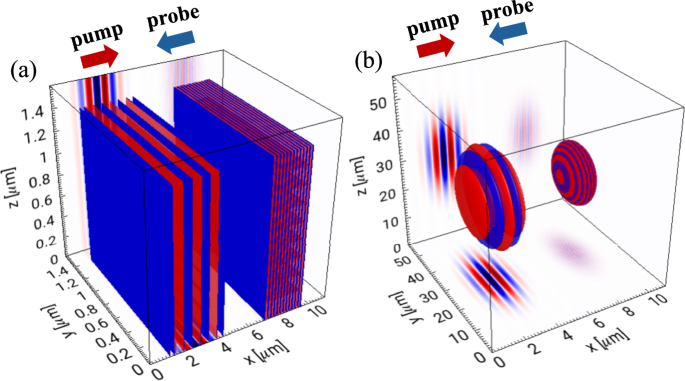
In vacuum birefringence4,5,6,7,8,9,10,11,12,13,14,15, a probe pulse travelling through a strong electromagnetic background will experience a change in its refractive indices along different polarisations. The difference in refractive indices leads to dephasing between the different polarisation components. A linearly polarised pulse will thus gain a small ellipticity in its polarisation after passing through the strong background. In our simulations, the strong field is provided by an ultra-intense pump pulse, and the birefringence is extracted from a probe pulse that passes through the pump pulse62,71. The two pulses will be counter-propagating along the \(\hat{{{{\bf{x}}}}}\)-axis, both focusing at the origin.
Consider two scenarios. In the first scenario, both the pump and probe pulses are plane waves with a Gaussian temporal profile71:
$${{{\bf{E}}}}({{{\bf{r}}}},t)=\bar{{{{\bf{E}}}}}\cos (kx\pm \omega t)\exp \left(-\frac{{(x\pm ct)}^{2}}{2{\sigma }^{2}}\right),$$
(10)
where E is the pump and probe electric field profile, \(\bar{{{{\bf{E}}}}}\) is the amplitude of the respective pulses, k and ω are their wave-numbers and frequencies, and σ is their longitudinal duration.
In the second scenario, both are finite-width Gaussian beams under the paraxial approximation72, with focus at the origin:
$${{{\bf{E}}}}({{{\bf{r}}}},t)= \,\bar{{{{\bf{E}}}}}\frac{{W}_{0}}{W(x)}\exp \left(-\frac{{y}^{2}+{z}^{2}}{{W}^{2}(x)}\right)\cos (\Phi ({{{\bf{r}}}}))\\ \times \exp \left(-\frac{{(x\pm ct)}^{2}}{2{\sigma }^{2}}\right),$$
(11)
where the phase Φ is given by
$$\Phi ({{{\bf{r}}}})=(kx\pm \omega t)+k\frac{{y}^{2}+{z}^{2}}{2R(x)}-\arctan \left(\frac{x}{{z}_{0}}\right).$$
(12)
W0 is the beam waist of the pulse. The transverse extent of the pulse and its focusing effect are described by a longitudinal distance-dependent width \(W(x)={W}_{0}\sqrt{1+{(\frac{x}{{z}_{0}})}^{2}}\), where \({z}_{0}=\frac{\pi {W}_{0}^{2}}{\lambda }\) is the Rayleigh range of the pulse.
In the expressions presented below, the subscripts 0 and p designate the relevant parameters for the pump and the probe pulse respectively. In both cases, \({\bar{E}}_{0}\gg {\bar{E}}_{{{{\rm{p}}}}}\), such that the birefringent effect created by the probe pulse is considered negligible. For a probe pulse that is initially linearly polarised at θ, it will acquire a phase difference between its two components along \(\hat{{{{\bf{y}}}}}\) and \(\hat{{{{\bf{z}}}}}\) after the interaction:
$${{{\bf{E}}}}_{{{{\rm{p}}}}}(x,t)=\frac{{\overline{E}}_{{{{\rm{p}}}}}}{2}\exp (-i\omega t)\exp (ik{\prime} x)\left[\cos (\theta )\exp (-i\Delta \phi ){{{{\bf{e}}}}}_{y}+\sin (\theta ){{{{\bf{e}}}}}_{z}\right]+\,{{{\rm{c.c.}}}}$$
(13)
where \(k^{\prime}\) is the wave-number of the pulse after it passes through the pump, and Δϕ is the phase difference given by62,71
$$\Delta \phi ({{{\bf{r}}}})=12{\pi }^{3/2}\xi {\overline{E}}_{0}^{2}{k}_{{{{\rm{p}}}}}{\sigma }_{0}\,{{{\rm{erf}}}}\left(\frac{x}{\sigma }\right)$$
(14)
for plane waves, and
$$\Delta \phi ({{{\bf{r}}}})=12{\pi }^{3/2}\xi {\widetilde{E}}_{0}^{2}({{{\bf{r}}}}){k}_{{{{\rm{p}}}}}{\sigma }_{0}\,{{{\rm{erf}}}}\left(\frac{x}{\sigma }\right)$$
(15)
for paraxial Gaussian beams. c.c. denotes the complex conjugate of the first term. The term \(\widetilde{{E}_{0}^{2}}\) given by
$${\widetilde{E}}_{0}^{2}({{{\bf{r}}}})=\frac{{\overline{E}}_{0}^{2}}{\left[1+{\left(\frac{x}{{z}_{0}}\right)}^{2}\right]}\exp \left(-2\frac{{y}^{2}+{z}^{2}}{{W}_{0}^{2}\left(1+{\left(\frac{x}{{z}_{0}}\right)}^{2}\right)}\right)$$
(16)
comes from a the modulus squared of the electric field strength of a transverse Gaussian profile. The longitudinal Gaussian profile integrates to the erf function. Finally, the ellipticity δ is related to the phase difference through
$$\delta =\frac{\sin 2\theta }{2}\widetilde{{E}_{{{{\rm{p}}}}}}\Delta \phi ,$$
(17)
where
$${\widetilde{E}}_{{{{\rm{p}}}}}({{{\bf{r}}}})=\frac{{\overline{E}}_{{{{\rm{p}}}}}}{\sqrt{1+{\left(\frac{x}{{z}_{{{{\rm{p}}}}}}\right)}^{2}}}\exp \left(-\frac{{y}^{2}+{z}^{2}}{{W}_{0}^{2}\left(1+{\left(\frac{x}{{z}_{{{{\rm{p}}}}}}\right)}^{2}\right)}\right).$$
(18)
An additional signature of the quantum vacuum present in the interaction of tightly focused Gaussian beams is the diffraction spreading of output photons due to momentum transfer from the pump beam, and has been studied in recent years in12,51,52,53,54. For the simulations presented here where a relatively loosely focused pump pulse was used (the simulated pump pulse has a Rayleigh range 100 times greater than that used in12), the momentum transfer effects are considered negligible.
Four-wave mixing
Now consider three input plane waves with frequencies and wavevectors (ωi, ki), where i = 1, 2, 3. An output beam whose four-wavevector (ω4, k4) satisfies the conservation of energy and momentum will be generated such that49:
$${{{{\bf{k}}}}}_{1}+{{{{\bf{k}}}}}_{2}={{{{\bf{k}}}}}_{3}+{{{{\bf{k}}}}}_{4},$$
(19)
$${\omega }_{1}+{\omega }_{2}={\omega }_{3}+{\omega }_{4}.$$
(20)
In the present work, a two-dimensional interaction geometry is considered, where the wavevectors of all four waves are confined to the \(\hat{{{{\bf{x}}}}}\)-\(\hat{{{{\bf{y}}}}}\) plane. The angles ϕi and γi are assigned to each field, where ϕi is defined as the angle k makes with the x-axis, and γi is the angle of polarisation from the z-axis, such that:
$${{{{\bf{k}}}}}_{{{{\bf{i}}}}}={k}_{i}\cos {\phi }_{i}\hat{{{{\bf{x}}}}}+{k}_{i}\sin {\phi }_{i}\hat{{{{\bf{y}}}}},$$
(21)
$${{{{\bf{E}}}}}_{i}({{{\bf{r}}}},t)={E}_{i}({{{\bf{r}}}},t)\left[\sin {\gamma }_{i}\sin {\phi }_{i}\hat{{{{\bf{x}}}}}-\sin {\gamma }_{i}\cos {\phi }_{i}\hat{{{{\bf{y}}}}}+\cos {\gamma }_{i}\hat{{{{\bf{z}}}}}\right].$$
(22)
Incoming beams are approximated as top-hat beams confined by length L, width and height b (L > b). It is further approximated that during the interaction process, the pulses interact in a cubic region with volume b3. The interaction region is assumed to exist for a limited period of time, determined by the duration of the pulse \(\frac{L}{c}\). Any edge-effects are considered negligible in the model. The output electric field then takes the form49
$${{{{\bf{E}}}}}_{{{{\rm{out}}}}}({{{\bf{r}}}},t)={E}_{0}(r,\theta ,\phi )\cos ({k}_{4}r-{\omega }_{4}t+\delta ){{{{\bf{G}}}}}_{{{{\rm{2d}}}}},$$
(23)
where
$${E}_{0}(r,\theta ,\phi )= \frac{1}{4\pi {\epsilon }_{0}}\frac{8\xi }{{k}_{4}\pi r}\frac{\sin \left({k}_{4}\frac{b}{2}(\cos {\phi }_{4}-\cos \phi \sin \theta )\right)}{\cos {\phi }_{4}-\cos \phi \sin \theta }\\ \frac{\sin \left({k}_{4}\frac{b}{2}(\sin {\phi }_{4}-\sin \phi \sin \theta )\right)}{\sin {\phi }_{4}-\sin \phi \sin \theta }\frac{\sin \left({k}_{4}\frac{b}{2}\cos \theta \right)}{\cos \theta }\\ {E}_{1}{E}_{2}{E}_{3},$$
(24)
r, θ and ϕ are conventional spherical coordinates, with the origin at the interaction centre. δ is a constant phase. G2d is a geometric factor that depends on the interaction geometry and polarisation of input pulses, and its full expression is given by Supplementary Note 1.
The output power can be calculated by integrating the intensity over a spherical shell, which gives
$${P}_{{{{\rm{out}}}}}=\frac{4{\xi }^{2}}{{c}^{2}{\epsilon }_{0}^{4}}{\left(\frac{1}{{\lambda }_{4}}\right)}^{4}{G}_{{{{\rm{2d}}}}}^{2}{\alpha }^{2}{P}_{1}{P}_{2}{P}_{3},$$
(25)
with α2 given by17
$${\alpha }^{2}= \frac{64}{{k}_{4}^{4}{b}^{6}}\int_{0}^{2\pi }\int_{0}^{\pi }\frac{{\sin }^{2}\left[{k}_{4}bf(\theta ,\phi )/2\right]{\sin }^{2}\left[{k}_{4}bg(\theta ,\phi )/2\right]}{{f}^{2}(\theta ,\phi ){g}^{2}(\theta ,\phi )}\\ \times \frac{{\sin }^{2}\left[{k}_{4}\frac{b}{2}\cos \theta \right]}{{\cos }^{2}\theta }\sin \theta \,d \theta \,d\phi ,$$
(26)
where \(f(\theta ,\phi )=1-\cos \phi \sin \theta\) and \(g(\theta ,\phi )=\sin \phi \sin \theta\). G2d is the modulus of G2d. P1,2,3 represent the power of the input pulses. The expected number of photons obtained per shot (Nout) is calculated by multiplying the power by the time duration and dividing by the output photon energy:
$${N}_{{{{\rm{out}}}}}=\frac{2{\xi }^{2}}{\pi {c}^{4}{\epsilon }_{0}^{4}\hslash }{\left(\frac{1}{{\lambda }_{4}}\right)}^{3}{G}_{{{{\rm{2d}}}}}^{2}{\alpha }^{2}L{P}_{1}{P}_{2}{P}_{3}.$$
(27)
Semi-classical QED solver
The Yee scheme73,74 is a widely used solver for Maxwell’s equations, wherein the electric and magnetic fields are computed on a staggered grid (See Supplementary Fig. anchorlinkdmmc11). To address the non-linearities in the modified Maxwell’s equations, the solver employs a modified Yee scheme62 (See Supplementary Fig. anchorlinkdmmc12 for a summary of the below process). At each time step tn:
-
The standard Yee scheme, based on the original Maxwell’s equations in the classical vacuum, is carried out to compute the electric and magnetic fields at staggered locations at tn+1.
-
Given that the non-linearities couple to all components of electromagnetic fields, the field values are linearly interpolated to all grid locations.
-
The two electromagnetic invariants, E2 − B2 and E ⋅ B are calculated at all grid locations at tn+1.
-
The effective polarisation (Eq. (7)) and magnetisation (Eq. (8)) are calculated at all grid locations at tn+1.
-
The electric field at tn+1 is then re-evaluated using the modified Ampere’s Law (Eq. (6)).
-
The updated electric field is used to revise the polarisation and magnetisation terms, which in turn update the electric field (Eq. (4)). The iterative process continues until convergence to the desired accuracy is achieved.
-
The magnetic field at tn+1 is then re-calculated using the modified Faraday’s Law (Eq. (4)).
This scheme has the important advantage that it can be straightforwardly incorporated into the electromagnetic solver in PIC code, and allows the calculation of quantum vacuum effects in the existing PIC code algorithm without significant modifications. The solver has been upgraded to be compatible with the latest version of OSIRIS, which supports new features such as non-paraxial pulses and pulse propagation at an angle75, and benefits from a shorter run-time. For the simulation of vacuum birefringence, a spatial resolution of \(\frac{1}{33}\) of the probe pulse wavelength is adopted along its propagation direction, and \(\frac{1}{15}\) of the beam width is used transversely. For four-wave mixing, to resolve the propagation of the pulses at an angle, the spatial resolution is set to \(\frac{1}{30}\) of the wavelength on the \(\hat{{{{\bf{x}}}}}\)-\(\hat{{{{\bf{y}}}}}\) plane, and \(\frac{1}{10}\) along \(\hat{{{{\bf{z}}}}}\). With the specified resolution, the simulation of vacuum birefringence with two plane-wave pulses took approximately 0.5 hour to complete without quantum effects, and 15 hours with the addition of the quantum vacuum solver, using the same computational resources. The simulations of four-wave mixing took 0.75 and 3.4 hours without and with the solver. The reasonable run-time allows for higher flexibility in running multiple simulations, for example when carrying out parameter scans.