Dynamics of domain walls
We consider two one-dimensional ferromagnetic tracks with mutual AF exchange coupling. Within each track, the initial classical magnetization configuration, M(x, t), at position x along the track and time t, is taken as a single steady DW, with their magnetizations being opposite in direction in the two tracks. After applying an AC current in x-direction to induce the AC staggered spin–orbit field (with amplitude proportional to current28 and frequency assumed to be the same as the AC current) that points in opposite directions in the two tracks at each time (see the “Methods” section), the dynamics of the x-component of the DW texture in the upper track, Mx, along the track as a function of time is illustrated in Fig. 1, highlighting the differences between periodic and chaotic states in an AF system under a time-oscillating staggered spin–orbit field. In this work, the current-induced spin-transfer torque is ignored, as its effect on DW motion is prevailed by the staggered spin–orbit field, as shown recently in ref. 16. Panel 1a shows a periodic state, where the DW oscillates regularly under a spin–orbit field amplitude of HSO = 74.5 mT with a period of 25 ps. The inset at the bottom of panel 1a illustrates the initial condition, depicting a 180° DW configuration and its associated topological charge Q defined by
$$Q=-\frac{1}{2\pi }\mathop{\int}\nolimits_{-\infty }^{\infty }\nabla \phi (x,t)\,{\rm {d}}x,$$
(1)
where ϕ(x, t) represents the angle of the magnetization in the plane of each track. This topological number counts how many times the magnetization wraps around the unit circle along the DW49, which is conserved during the time evolution of the system, ensuring that the DW structure is topologically protected and maintains its stability against external perturbations.
Fig. 1: Dynamic states of domain walls.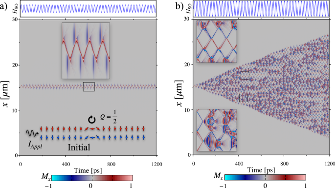
a Dynamics of Mx along the upper track as a function of time for a periodic state, with the value represented in a color gradient (gray near Mx = 0, pink near Mx = 1, and cyan near Mx = −1). The upper panel shows the applied spin–orbit field HSO = 74.5 mT with a period of 25 ps. The lower inset illustrates the initial condition of the system, obtained by relaxing the domain wall, as well as the value of its topological charge (Q = 1/2) and the form of the AC current applied along the x-axis (IAppl). The middle inset displays a magnified view of the oscillations in the DW, revealing the emission of spin waves due to the relativistic contraction of DWs. b Dynamics of the Sx component along the track as a function of time for a chaotic state. The upper section shows the applied spin–orbit field HSO = 78.0 mT with a period of 25 ps. A nucleation process is observed when the DW reaches its maximal group velocity, causing the DW to contract following Lorentz transformations until a point where nucleation occurs, giving rise to new DWs while maintaining the same topological charge. The middle insets show magnified views of the DW proliferation process. The conservation of Q ensures that, despite the creation and annihilation of multiple DWs, the total topological charge of the system remains constant, which is fundamental for the integrity of the system.
The upper inset in the gray area of Fig. 1a reveals a magnified view of the DW oscillations, showing the emission of spin waves. These periodic oscillations lead to spin wave emissions due to Lorentz contraction, which transports energy and angular momentum across the system. According to Shiino et al.10, as the DW velocity approaches the maximal group velocity of spin waves, vg, Lorentz contraction induces spin wave emission in the terahertz frequency range. The relativistic contraction of DW width Δ is described by
$$\Delta (v)={\Delta }_{0}\sqrt{1-{\left(\frac{v}{{v}_{{\rm{g}}}}\right)}^{2}},$$
(2)
where Δ0 = 19.8 nm corresponds to the DW width in the static state. This equation illustrates that as the DW velocity increases, its width Δ(v) decreases. This contraction is evident in the periodic oscillations as shown in the upper inset in the gray area of Fig. 1a, where the width of the red-colored region along the y-axis is larger near the motion-reversal instants at which DW velocity is smaller. The spin wave emission is also clearly observed in this simulation result. This approach highlights the connection between topology and the dynamics of DWs in AF systems, similar to what is observed in ferromagnetic systems.
Figure 1b shows a chaotic state induced by a spin–orbit field amplitude of HSO = 78.0 mT with the same current oscillation period. In this regime, a complex behavior is observed where the initial DW undergoes nucleation and proliferation of new DWs. The dominant energy of the DW texture relevant to its width comes from ferromagnetic exchange (∝JF) plus easy-axis anisotropy (∝K2⊥) energies along the track and can be written as E = (γ + 1/γ)E0 with \({E}_{0}\propto \sqrt{{J}_{{\rm{F}}}{K}_{2\perp }}\propto {J}_{{\rm{F}}}/{\Delta }_{0}\propto {K}_{2\perp }{\Delta }_{0}\) and \(\gamma =1/\sqrt{1-{v}^{2}/{v}_{{\rm{g}}}^{2}}\) is the Lorentz factor. At the initial static state, γ = 1 and the energy is 2E0. When the DW starts to move with Lorentz width contraction, γ increases from 1 and the energy increases from 2E0. Together with the energies created by the emitted spin waves, the accumulated energy increments until a critical point results in the DW breaking and subsequent nucleation of new DWs. This process reflects the dynamical instability in the system, where accumulated energy is released to create new domain structures. This instability is analogous to Walker-like breakdown in antiferromagnets, where a DW reaches a critical velocity that destabilizes its structure, leading to the formation of new magnetic textures. In our case, as the DW accelerates toward the magnonic limit, its width undergoes relativistic Lorentz contraction, concentrating energy until a threshold is exceeded, triggering the generation of soliton–antisoliton pairs and ensuring the conservation of topological charge. This mechanism has been reported in Otxoa et al.15, where it is shown that in this highly nonlinear regime, some DWs can even reach supermagnonic velocities, exceeding the theoretical magnonic speed limit due to the breakdown of Lorentz invariance in the system’s dynamics.
This phenomenon is distinct from spin wave emission since it involves the physical reconfiguration of DWs. Although spin waves do not directly cause nucleation, they influence this process by modulating local energy distribution along the track. Spin waves can interfere constructively or destructively, creating regions of high or low energy that affect DW stability and rupture points. This effect is evident in the figures, particularly in Fig. 1b, where the magnified view in the lower left corner highlights the spin wave emissions that precede the nucleation of new DWs. Frequent DW collisions occur in the chaotic state, reconfiguring DWs, altering their trajectories and velocities, and potentially leading to new DW nucleation if collision energy is sufficient to overcome local energy barriers. The figures show areas where contour lines meet and mix, indicating DW collisions and reconfigurations. The energy distribution due to spin waves is crucial in DW dynamics, as spin waves act as an additional energy dissipation channel, allowing DWs to release accumulated energy. However, when this dissipation is insufficient, the remaining energy can lead to DW rupture and nucleation. The balance between spin wave emission and DW nucleation defines the complexity of the chaotic state observed.
In summary, Fig. 1 provides a comprehensive view of the transition between periodic and chaotic DW behavior in an antiferromagnetic system under an applied spin–orbit field. The distinction between spin wave emission and nucleation processes is clearly highlighted, offering a deep understanding of the dynamic mechanisms involved. Periodic oscillations result in spin wave emission that dissipates energy, whereas in the chaotic state, energy accumulation leads to DW rupture and nucleation. DW collisions and the influence of spin waves on energy distribution add another layer of complexity to the system’s dynamics.
In order to capture the details of spatio-temporal dynamics of the system of DWs combined with spin waves, we use fast Fourier transform (FFT) to analyze the magnetizations as follows. Figure 2a, b are enlarged views of Mx corresponding to the periodic state in Fig. 1a and the chaotic state in Fig. 1b, respectively. In Fig. 2a, stable dynamics are observed as the spin wave emission occurs in a repetitive manner in time with a fixed period. The FFT of time evolution of Mx at each position into frequency-space is shown in Fig. 2b, displaying distinct peaks characteristic of periodic motion. Specific oscillation nodes are observed, indicating both spatial and temporal regularity in the system. To confirm this expectation, the time evolution of Mx averaged along the entire track is shown in Fig. 2c, and regular oscillations synchronized with the applied field are observed. The FFT of the spatially averaged Mx presented in Fig. 2d corroborates the periodic magnetization oscillations in time with a pattern of regular peaks in the frequency domain highlighting the deterministic behavior of the DW dynamics.
Fig. 2: Soliton proliferation.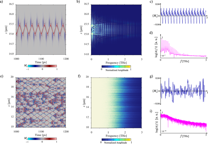
a Dynamics of Mx along the upper track as a function of time for a periodic state as an enlarged view of Fig. 1a. b Fast Fourier transform (FFT) of the temporal evolution of Mx(x, t) at each spatial position from panel (a), transforming the time-space data into frequency-space. Periodic nodes are observed in both time and position. c Mean value of Mx along the upper track as a function of time, showing the stability of the dynamics in the periodic state. d FFT of the mean value of Mx, indicating global periodic behavior. e Enlarged view of Mx for the chaotic state in Fig. 1b. f FFT of Mx in panel (e), showing a broad spectrum of frequencies characteristic of chaotic dynamics. g Mean value of Mx as a function of time for the chaotic state, highlighting the complexity of the dynamics. h FFT of the mean value of Mx, revealing the broad frequency spectrum typical of chaotic states.
On the other hand, Fig. 2e depicts the dynamics of Mx in a chaotic state. The dynamics reveal the proliferation and annihilation of DWs and their complex interactions, indicating chaotic behavior in both space and time. The FFT of Mx is presented in Fig. 2f, revealing peaks smeared in a broad and continuous distribution of frequencies, which is typical of a chaotic state that reflects the irregular and non-repetitive nature of magnetization dynamics. This complexity in the frequency domain indicates the absence of a dominant pattern and shows a superposition of multiple oscillation modes that are interacting nonlinearly. This chaotic dynamics is highly sensitive to initial conditions and external perturbations. The presence of multiple peaks in the FFT spectrum suggests the existence of various temporal and spatial scales in the DW dynamics. The spatial average of Mx being irregular in time as shown in Fig. 2g again confirms this behavior. The FFT of this average value, presented in Fig. 2h, reveals a broad and complex frequency spectrum, indicating the nonlinear and chaotic dynamics of the system.
Figure 3 illustrates the phase transitions of the dynamics of our AF DWs represented by a bifurcation diagram. To survey the dependence of magnetization dynamics on the excitation spin–orbit field, we calculate two primary dynamic indicators as the growth rate of new DWs, ξ, and the complexity, C, which allow us to characterize the transition between periodic and chaotic states as a function of various field amplitudes HSO from 65 to 85 mT in an interval of 0.5 mT, and periods T = 15, 20, 25, 30 ps. In Fig. 3a, we illustrate the chaotic dynamics of the DWs and their proliferation process. An analogy can be drawn to the turbulence model in fluid mechanics, where magnetic textures proliferate in space and time in a manner similar to vortexes in a turbulent fluid. This detailed view enables us to clearly observe the complex interactions and reconfiguration of the DWs. In Fig. 3b, we present the number of detected DWs as a function of time, represented by blue points. The pink points indicate the moving average of the number of DWs, calculated by averaging over a window of 100 time steps starting just when the DWs begin to nucleate that is, after a transient period during which the DW still oscillates without nucleation. This approach allows us to smooth out rapid fluctuations and highlight general trends in the proliferation of DWs. The green line shows a linear fit of these averaged points. The observed fluctuations highlight the nucleation and annihilation processes of DWs, emphasizing the nonlinear dynamics of the system.
Fig. 3: Phase diagram.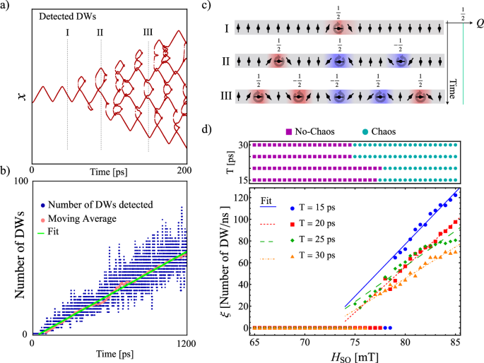
a Illustration of the chaotic dynamics of the DW and its proliferation process, using an analogy with the vortex model in fluid mechanics. This model facilitates the visualization and understanding of the complexity of DW behavior in the AF system. Labels I–III indicate specific moments at which the topological configuration is schematically shown in panel (c). b Number of DWs detected as a function of time. The blue points represent the number of DWs detected at each time instant. The pink points show the moving average of the number of DWs, which smooths out fluctuations and allows for a better interpretation of the overall trend. The green line is a linear fit of the moving average points, indicating the growing trend of the number of DWs over time. c Topological configuration of the DWs at instances I–III marked in panel (a). Each row shows the DWs at different time instants, highlighting the conservation of the topological charge Q. The numerically extracted time dependence of the topological charge is illustrated on the right side of the panel, showing that Q is conserved over time despite the proliferation of new DWs. The color code represents the magnitude of Mx with blue for Mx = −1, red for Mx = 1/2, and gray for Mx = 0. d Bifurcation diagram representing the DW nucleation rate ξ as a function of the spin–orbit field strength HSO and oscillation period T. The nucleation rate ξ is extracted from the slope of the linear fit of the moving average in panel (b), which quantifies the growth rate of the number of DWs per unit time. The spin–orbit field strength is varied from HSO = 65 mT to HSO = 85 mT in steps of ΔHSO = 0.5 mT for four different excitation periods T, allowing us to track the transition in nucleation dynamics. The upper section of panel (d) presents a phase diagram characterizing the transition between periodic and chaotic behaviors based on the complexity indicator C. Purple squares correspond to C = 0, indicating periodic dynamics, whereas green circles represent positive complexity values, signaling chaotic behavior. This classification reveals how the system transitions between periodic and chaotic regimes as HSO and T are varied.
Figure 3c shows the topological configuration of DWs at three instants labeled by I–III in Fig. 3a. Above each DW texture, their topological charge Q is indicated, revealing that DWs are produced in pairs with opposite topological numbers, such that the net Q is conserved in time as shown in the right panel of Fig. 3c. Hence, despite the chaotic proliferation and complex dynamics, the system remains in the same topological class at all times.
Figure 3d presents a characterization of the dynamical behaviors of the system based on two complementary indicators: a bifurcation diagram (lower panel) and a phase diagram (upper panel). These indicators provide insight into the transitions between periodic and chaotic regimes in the DW dynamics as a function of the spin–orbit field amplitude HSO and the oscillation period T. The lower panel of Fig. 3d displays the bifurcation diagram, where the DW nucleation rate ξ is extracted from the slope of the linear fit of the moving average in Fig. 3b. This slope quantifies the growth rate of the number of DWs per unit time. The spin–orbit field strength is varied from HSO = 65 mT to HSO = 85 mT in steps of ΔHSO = 0.5 mT for four different excitation periods T. The linear fits reveal that the nucleation rate follows a proportional trend with the field amplitude, expressed as ξ = aiHSO + bi. The values of ai, which represent the sensitivity of the nucleation rate to variations in HSO, are given by ai = {10.538, 7.86, 6.78, 5.56} mT−1 for T = {15, 20, 25, 30} ps, respectively. The bifurcation diagram allows us to track the transition from a periodic to a chaotic regime, where ξ = 0 corresponds to a periodic state with no nucleation, and ξ > 0 indicates the onset of chaotic proliferation of DWs.
The upper panel of Fig. 3d presents a phase diagram where the complexity indicator C is used to distinguish between periodic and chaotic dynamics. The classification is performed using two distinct markers: purple squares represent C = 0, indicating periodic dynamics, while green circles correspond to positive complexity values, signaling chaotic behavior. The complexity measure, which combines entropy and disequilibrium, quantifies the degree of order in the system (see Supplementary Material for details)50. The diagram reveals that the system exhibits a transition between periodic and chaotic regimes as a function of both HSO and T, with lower T values favoring a chaotic response. Interestingly, despite the strong correlation between the complexity C and the nucleation rate ξ, certain regions in the diagram show cases where ξ = 0 while C > 0, indicating that the system remains chaotic even when no new DWs are nucleated. This suggests that the magnetization dynamics can retain chaotic features without additional DW proliferation, highlighting the intricate interplay between topological excitations and dynamical complexity in the system.
Altogether, Figs. 1–3 offer a comprehensive view of how the AC staggered spin–orbit field influences both the nucleation rate and complexity of the system to induce the phase transition of the DW configuration and dynamics between periodic and chaotic phases. The nucleation process we observe is neither linear in time nor predictable, as it depends on local fluctuations of energy. The instability suffered by the relativistically moving DW disturbs its regular motion and texture, and eventually producing spin waves and new DWs to release energy, which interact with each other nonlinearly. This creates an environment where small variations can generate significant changes in the system dynamics and result in chaotic behavior. In summary, the interplay of relativistic contraction, energy accumulation, and nonlinear interactions between DWs and spin waves induces chaotic dynamics during the nucleation process. This is reflected in the positive complexity observed in chaotic states, even in the absence of new DW proliferations. In these cases, chaos manifests through irregular and sensitive movements of the existing DWs, induced by nonlinear interactions and energetic fluctuations, without necessarily involving additional nucleations.
These observations not only deepen our understanding of chaotic DW dynamics but also provide insight into their potential functional implications. These results reinforce our understanding of how relativistic contraction, spin wave emissions, and nonlinear interactions collectively regulate the stability of domain walls in antiferromagnetic systems. The transition between periodic and chaotic regimes, quantified through complexity measures and DW proliferation rates, highlights the fundamental role of energy accumulation and dissipation in the evolution of these magnetic textures. Beyond its theoretical significance, the ability to induce and control chaotic dynamics in these systems suggests that these phenomena could be leveraged in advanced spintronic applications, such as the development of magnonic architectures requiring highly nonlinear and adaptive responses.
Reservoir computing
After investigating the chaotic DW proliferation driven by staggered spin–orbit field in AFMs, in this section, we propose the potential of a proliferated multiple-DW configuration as a viable system for spintronics reservoir computing (RC) by demonstrating the possession of short-term memory and nonlinearity inherent in the magnetization responses to external spin–orbit field inputs in this system. We consider two one-dimensional ferromagnetic layers with mutual AF exchange coupling, as illustrated in Fig. 4a. Each layer has a length of 6000 sites and contains seven equally spaced DWs with centers located at site indices 750n with n = 1, 2, …, 7 (see Fig. 4b). Each neighboring DWs have opposite winding numbers, mimicking the texture generated by the chaotic proliferation from a single seed DW that preserves the topological number. We evaluate the performance of this system on two benchmark tasks of RC as the short-term memory (STM) and parity-check (PC) tasks31,34,41.
Fig. 4: Schematics RC.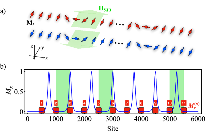
a Schematics of the bilayer AF-DW system for RC. Black arrows indicate the local magnetization vectors and the green thick arrows are the local input SO-fields. b Initial configuration of the x-component of the DW magnetizations in the upper layer (blue curve). For the lower layer, the sign of Mx is the opposite. Green shaded zones are input areas and the eleven detectors are labeled by red boxes.
For both tasks, the input data sin(Ti) consists of a sequence of random digits, either 1 or 0, at integer time steps Ti. The goal of RC by using this DW system is to predict specific transformations of the inputs by an output function, taken as a linear combination of the magnetization responses measured on local areas in the DW-array. The correspondence between input digits and physical excitations in the DW system is designed as follows. When sin(Ti) = 1, we simultaneously apply three local staggered spin–orbit field pulses in ±y-direction for the upper and lower DW array, respectively. These pulses are applied to three input areas located on site indices from 1001 to 1500, 2500 to 3000, and 5001 to 5500, as indicated by green areas in Fig. 4b. When sin(Ti) = 0, we reverse the directions of the spin–orbit field pulses for both layers and apply them on the same local areas with the same pulse width. The surveyed pulse width of spin–orbit field ranges from 0.1 to 0.5 ps, while its magnitude is varied from 10 to 60 mT in this study.
We placed 11 detectors on the DW array as shown in Fig. 4b. In the area of each detector, the averaged magnetization at a number of virtual-node temporal instants in each spin–orbit field pulse is recorded to define the reservoir state vector. A linear transformation of the measured magnetizations is defined as an output function, with the coefficients being the weight vector components being optimized to minimize the mean square error between the target and output for a training set of random digits. The optimized weight vector is then taken to predict another testing set of digits by their magnetization responses (see details in the “Methods” section). The target functions for STM and PC tasks are respectively defined in Eqs. (6) and (7) in the “Methods” section. From these definitions, the STM task investigates to what extent the input at a previous time Ti −Tdelay can be reconstructed by the reservoir state at current time Ti, which is important for applications such as sentence prediction and speech recognition45,46,47 that involve time-series data. Meanwhile, the PC task examines to what extent the reservoir can nonlinearly transform its components into a summation of past inputs modulo 2, which is essential for problems like pattern classification and hand-written digit recognition42,43,44 that require nonlinearity.
After the training procedure, the squared correlation between the testset targets and outputs for each detector is calculated. As shown in Supplementary Fig. 4, empirically we find when a detector is placed close to both the edge of any input areas, and either to one of the DW centers (e.g., detectors 3 and 6 in Fig. 4b) or near the system edge (e.g., detectors 11), a better-squared correlation is obtained for both tasks. This indicates the need for both a large spatial gradient of HSO and either a large gradient of My or strong spin wave reflection near the system edge, to excite significant magnetization responses that possess memory and nonlinearity relative to the input. To quantify the performance, we calculate the capacities CSTM(PC) for STM (PC) tasks31,34,41 for better detectors 3, 6, and 11, defined as the sum of the squared correlations from Tdelay = 1 to 30. A larger capacity indicates a better performance by the reservoir. We note that in literature many works calculate the capacity including the point of Tdelay = 0. Since the squared correlation at Tdelay = 0 is trivially close to 1, we exclude this point to estimate the capacity in a stricter way, following ref. 34. We achieve the highest CSTM and CPC values of approximately 10.5 and 1.5, respectively, comparable with other spintronics reservoirs using a similar number of virtual nodes 31,34,36,41. This finding clearly demonstrates the potential of a multiple-DW array proliferated by spin–orbit field in AFMs for applications in physical reservoir computing. We have tested the reproducibility by performing sequential runs of the tasks and compared the performances between the proposed multiple-DW array and a pure AF state without DW textures and find the multiple-DW array shows much better results (see the “Methods” section for details).
To investigate the potential input dependence of the performance, we compare the capacities carried out by different components of magnetizations under varying pulse widths and amplitudes of spin–orbit field, as illustrated in Fig. 5. In Fig. 5a, the pulse width is fixed at 0.2 ps for all curves. The results show that increasing the field amplitude from 10 to 60 mT does not significantly change the capacities. For HSO = 10 mT, the capacities carried out by Mx and My components were lower than those for higher SO-field amplitudes. Interestingly, the data reveals a contrasting behavior between the STM and PC capacities. Specifically, the Mz component has roughly better results for STM capacities compared to Mx and My. On the contrary, for PC capacities, Mz is worse than the other components. This opposite behavior between STM and PC capacities is reminiscent of the empirical law of memory-nonlinearity trade-off51,52, which is frequently observed in dynamical models or physical systems in RC, suggesting that the introduction of nonlinearity into reservoir dynamics tends to degrade memory capacity.
Fig. 5: RC results.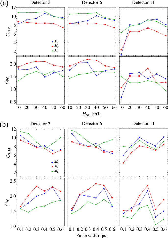
Comparison of the capacities as functions of a SO-field amplitude and b SO-field pulse width for the three best detectors: 3, 6, and 11.
In Fig. 5b, we study how the capacities for STM and PC tasks change with different pulse widths, ranging from 0.1 to 0.6 ps. For detectors 3 and 6, as the pulse width increases from 0.1 and 0.4 ps, the STM capacities tend to decrease, while the PC capacities increase. This opposite behavior is another indication of a memory-nonlinearity trade-off, where an increase in one capacity typically leads to a decrease in the other. However, detector 11 exhibits a unique behavior. As the pulse width increases, both STM and PC capacities follow a similar trend, which violates the expected trade-off. This suggests that for detector 11, it may be possible to simultaneously enhance the short-term memory and nonlinearity by fine-tuning the input pulse width. This capability is particularly advantageous for machine-learning tasks since many realistic problems require both memory and nonlinearity. The common trade-off between memory and nonlinearity limits the learning potential of reservoirs, making our finding significant. This distinct behavior of detector 11 as compared to detectors 3 and 6 may be attributed to the edge effects of the system. These edge effects might enhance both memory and nonlinearity due to phenomena like spin wave reflection and interference occurring near the system edge. It is left for our future work to find concrete ways to overcome the memory-nonlinearity trade-off and to enhance capacities for both STM and PC tasks in this multiple-DW reservoir.
The results presented in this work demonstrate the strong potential of DW-based reservoirs in antiferromagnetic systems, where the interplay between chaotic DW dynamics and spin wave interactions enables efficient and tunable computational performance. The ability to reconfigure the reservoir by adjusting the amplitude and period of the spin–orbit field provides a mechanism to optimize memory and nonlinearity trade-offs, a fundamental challenge in RC. Furthermore, our findings highlight how the mechanisms governing chaotic DW proliferation, previously analyzed in detail, play a crucial role in enhancing the diversity and richness of dynamical responses in the reservoir. This connection between DW chaos and computational capacity suggests that DW proliferation dynamics could be leveraged to improve the performance of physical reservoirs in spintronic systems. While these results represent an initial step, future research could explore strategies to optimize the interaction between DW dynamics and input parameters, with the goal of enhancing the efficiency and stability of these systems in neuromorphic computing applications.