Observations and data reduction
Our astronomical monitoring targeting the microquasar GRS 1915 + 105 was conducted using the FAST. The primary observation employed tracking mode through the central beam of the 19-beam receiver, operating within the nominal 1–1.5 GHz frequency range, while the 50 MHz bands at both spectral boundaries need to be excluded. This observation started at 01:35:00 UTC on January 25, 2021, sustaining data collection for 90 minutes with a 98 microseconds temporal resolution. The field of view of the central beam is ~2.9 arcminutes. For calibration purposes, periodic noise injections (0.210326592 seconds) were conducted in five-minute intervals both preceding and following the source tracking observation. High power noise diode mode was used in our observations for calibration, in which the noise and noise temperature are 100% linear polarized and 12.5 K, respectively.
The observational data of FAST are stored in the standard PSRFITS format56. Our data reduction pipeline starts with the preprocessing of FITS file using astropy package57. The preprocessing involves two operations: (1) systematic re-sampling of the original data across full 4096 frequency channels and 128 subints, (2) concatenating the re-sampled preprocessed data files. The PRESTO software suite performs subsequent analysis on the merged data file, generating an uncalibrated lightcurve time series and radio frequency interference (RFI) mitigation mask through automated detection. The common detected interference patterns include the strong noisy signal in the periodogram (such as 50 Hz alternating current noise and its harmonics persisting throughout observations), non-negligible short-time spikes caused by noise in channels 650–820 (1080–1100 MHz), and broadband RFI peaks around channels 1500–2200. Following standard RFI mitigation protocols, we excluded these affected spectral regions from our analysis. The processed time series, now cleansed of these interference components, contains relative flux intensity measurements ready for subsequent calibration.
Flux density calibration
The temperature of the observed source in the on-off mode is
$${T}_{src}(t)={T}_{cal}\cdot \frac{ON}{ONCAL-ON}-{T}_{sys}(t),$$
(1)
where Tcal is the temperature of the injected reference signal from the noise diode, ON and ONCAL are the intensity values in the turning-off and turning-on states of the noise diode, respectively, when the telescope is directed at the celestial source in the on-off mode for the calibration scans before and after the tracking observations, and Tsys(t) is the time-dependent system temperature of the telescope when the telescope is pointing at the background sky, which is given by
$${T}_{sys}={T}_{cal}\cdot \frac{OFF}{OFFCAL-OFF},$$
(2)
OFFCAL and OFF are the intensity values in the turning-on and turning-off states of the noise diode, respectively, when the telescope is directed at the background sky.
Then the flux density can be calculated by the following formula,
$$Flux(t)=\frac{I(t)-OFF}{ON-OFF}\cdot {T}_{src}(t)\cdot \frac{1}{G},$$
(3)
where I(t) is the observed intensity value from the telescope with time in the tracking mode observations, G = ηG0 differs from the measured gain G0 = 25.6 K/Jy by a factory η, is the full gain of FAST in the sky coverage, η is the aperture efficiency58.
Polarization calibration
The original data files are processed using DSPSR59 and PSRCHIVE56, with each file folded over its own duration to extract four time series corresponding to the recorded Stokes parameters. These are denoted as \({I}_{1}^{2}\), \({I}_{2}^{2}\), CR, and CI60, where CR and CI represent the real and imaginary components of the complex product I1*I2. In practical observations, the feed systems are seldom ideal, and two main instrumental effects relative gain imbalance (often referred to as leakage) and channel phase offset must be accounted for through calibration. The observed and calibrated Stokes vectors are indicated by the subscript o and c respectively, are typically related via the system s Mueller matrix61,62. Thus we have,
$$\begin{array}{r}{S}_{o}={{{\mathcal{M}}}}\times {S}_{c}=\left[\begin{array}{cccc}1&f&0&0\\ f&0&0&0\\ 0&0&cos2\delta &-sin2\delta \\ 0&0&sin2\delta &cos2\delta \end{array}\right]\times {S}_{c}\end{array}$$
(4)
where \({\prime}\) means the injected reference signal, and the leakage \(f=\frac{{Q}_{o}^{{\prime} }}{{I}_{o}^{{\prime} }}\). We calibrated the phase error as \({\delta }^{{\prime} }=\frac{1}{2}\arctan \frac{{V}_{o}^{{\prime} }}{{U}_{o}^{{\prime} }}\), then removing the error from orientation, we can get the calibrated values of the four Stokes parameters:
$$\begin{array}{rcl}{I}_{c}&=&\frac{{I}_{o}\, -\, f \,*\, {Q}_{o}}{1\, -\, {f}^{2}}\hfill \\ {Q}_{c}&=&\frac{{Q}_{o}\, -\, f \,*\, {I}_{o}}{1\, -\, {f}^{2}}\hfill \\ {U}_{c}&=&P\cos 2\delta \cos 2{\delta }^{{\prime} }+P\sin 2\delta \sin 2{\delta }^{{\prime} }\hfill \\ {V}_{c}&=&P\sin 2\delta \cos 2{\delta }^{{\prime} }+P\cos 2\delta \sin 2{\delta }^{{\prime} },\end{array}$$
(5)
where \(P=\sqrt{{U}_{o}^{2}+{V}_{o}^{2}}\). Finally, the degrees of linear and circular polarization, and polarization position angle are calculated as
$$LP=\frac{\sqrt{{Q}^{2}+{U}^{2}}}{I},\quad CP=\frac{V}{I},\quad PA=\frac{1}{2}\arctan \frac{U}{Q}$$
(6)
Periodicity studies
The main aim of the timing analysis here is to search for the quasi-periodic oscillations (QPOs) ranging from ~1−100 s in the light curves of both radio flux density and polarization parameters. QPOs are generally studied in the Fourier domain and show up in the power density spectrum as narrow peaks. We used Numpy.fft.fft and Stingray in Python packages to perform the power density spectrum (PDS) analysis, including the production and fitting of the PDS.
The PDS calculated with the packages mentioned above is the Fourier transform of the light curve and is unnormalized. In X-ray observations, such PDS need to be normalized so that the evolution of the QPO can be studied by computing some physical quantities such as the QPO factor for observations of the same QPO but in different equipments. However, unlike the photon number distribution in X-ray observations, the flux density observed in the radio band is highly related to instrument response, system noise, and so on. In order to facilitate the adjustment of fitting parameters and the generation of dynamic PDS, the following procedures are performed: when computing the PDS, we treat the flux density in the radio band as the number of photons in X-ray observations, and then normalize the PDS with the Leahy and rms normalizations. When computing the dynamic PDS, we divide the light curve into segments of 200 s duration and calculate the PDS independently for each segment. To minimize the inaccuracy caused by such crude segmentation and the distortion to the light curve structures, each segment is shifted in 80 s steps.
Wavelet analysis is a valuable approach for analyzing time series having a wide range of timescales or variations which would decompose the time series into time-frequency space, so that we can check both the dominant modes of variability and how those modes vary in time63. In reality, wavelet analysis would also perform the FFT of time series. Unlike traditional FFT for PDS, wavelet analysis would use wavelet functions with different time and amplitude scales for further analysis; however, the most important feature of wavelet analysis is that it would assume a background noise at different scales, which would be useful for calculating the 95% confidence contour. Meanwhile, the shortcomings of dynamic PDS which are inevitable would not appear in wavelet analysis. But the mother wavelet utilized in analyzing processing might have a considerable impact on the end outcome, such as how ‘Morlet’ provides better temporal localization, whereas ‘Paul’ provides better frequency localization. Wavelet analysis, however, has been applied to the timing analysis of X-ray light curves in some X-ray binaries64,65.
For wavelet analysis in our data, we have used the ‘Morlet’ wavelet function for analysis and taken red noise into account in wavelet analysis by calculating the correlation functions of the time series. A simple model to compute red noise is the univariate lag-1 autoregressive process, so that we estimate the red noise from \(({\alpha }_{1}+\sqrt{{\alpha }_{2}})/2\), where α1 and α2 are the lag-1 and lag-2 autocorrelations of the time series. On the other hand, the wavelet analysis would also give the significance levels of the power spectrum based on the red noise model63. In our results (see Fig. 4), the regions enclosed by black solid curves and colored with blue denote the promising signals whose confidence levels are higher than 95%. The result of wavelet analysis would clearly show the evolution of periodic signals both in the time and frequency domains.
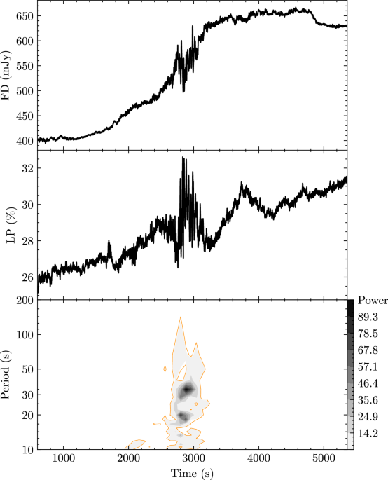
At first, we calculated the power density spectrum for every two hundred seconds data set of the calibrated flux time series, checking the possible periodic signals in the PDS, then we arranged them in chronological order to get a set of spectra which is called the dynamical power spectrum (see Fig. 1 for the whole observational time series on January 25 2021). For the most observational time regimes, there are no periodic signals detected in the dynamical PDS, while only for the time interval from 2700−3100 s when the flux density was still increasing near to the peak, there existed the multiple periodic signals at 17 and 33 s. We also presented the average power density spectrum of the calibrated flux density light curve (see the PDSs in Fig. 3) from the observed time interval from 2400 s to 3200 s. The periodic peaks around 17 and 33 s have significance levels higher than 5σ based on the light curve simulation algorithm66, in which we have simulated 20000 light curves with power-law distributed noises appropriate for our data and re-sampled these light curves to ensure the resolution that matched our observation data.
In Fig. 3, we also present the PDSs for the light curves of three polarization parameters (LP, CP and PA). The LP light curve shows similar variation patterns of the flux density and has significant QPO signals at the periods of 17 and 33 s (> 5σ). The CP and PA light curves exhibit very weak QPO signals, with periods of ~50 s, 30 s, and 20 s for CP, and 40 s, 30 s, and 15 s for PA. All possible PDS peaks detected in both CP and PA have low significance levels (below or around 3σ). Therefore, the light curve of LP shows similar variation patterns with that of flux density. The CP and PA curves would have similar variation patterns, but are quite different from the curves of both flux density and LP.
Then, wavelet analysis for flux and polarization parameters has also been conducted. The results are shown in Fig. 4, in which the light-yellow regions and the red dashed curves mark the ’cone of influence’ due to edges effects, the blue regions enclosed by red solid curves suggest the existence of promising signals with their confidence levels are higher than 95 %. Meanwhile, the blue dash-dotted horizontal lines in Fig. 4 represent the positions of the two periodic signals for flux and LP light curves (17 and 33 s) in the wavelet analysis results. For a more profound comprehension of the wavelet results as shown in Fig. 4, one may regard Fig. 4 as results of dynamic PDS calculated by FFT, with abscissa and ordinate indicating the time and period (frequency) domains. The reason of selecting wavelet for timing analysis stems from its ability to dynamically adapt the scale of the mother wavelet according to the local features of the signal. In contrast to traditional FFT, the wavelet analysis method can effectively avoid the negative impact of signal discontinuity caused by truncation, enabling a more accurate and flexible reflection depiction of the signal’s instantaneous features and abrupt changes. In our wavelet results, the high time-resolution power density with time shows more details of the variations for these periodic oscillation signals. The strongest period modulation of 33 s appeared near 2760 s in both total flux density and LP light curves, but could not be seen at 3050 s. The signal at 17 s is relatively weak and has similar time intervals to the 33 s signal. The light curve of CP shows the strong periodic signal at ~50 s from 2600 s–2800 s, while has a possible 25 s period from 2800 s to 2900 s. And PA also shows the periodic signal around 40–50 s from 2800 s to 2900 s.
Correlation analysis
The light curves in the Figure 2 clearly illustrate an anti-correlated relationship between flux density and linear polarization during the oscillation stage: the peaks of the flux always correspond to the valleys of the LP. We use linear regression analysis on flux density and linear polarization to confirm this anti-correlation.
Pearson correlation coefficient (PCC) is the best method for measuring the magnitude of the linear association between variables since it is based on the utilization of covariance and is defined as:
$$\begin{array}{l}{\rho }_{X,Y}=\frac{cov(X,Y)}{{\sigma }_{X}{\sigma }_{Y}},\end{array}$$
(7)
where ρX,Y is the PCC and on or between −1 and + 1, and σX and σY are the standard deviations of X and Y, respectively. Since cov(X, Y) is the covariance of variable X and Y, so the formula of PCC can be written as:
$$\begin{array}{l}{\rho }_{X,Y}=\frac{{\mathbb{E}}[(X\, -\, {\mu }_{X})(Y\, -\, {\mu }_{Y})]}{{\sigma }_{X}{\sigma }_{Y}}\end{array}$$
(8)
We used the Seaborn and SciPy.stats in Python package to do the linear regression analysis and the PCC calculation. In addition, we performed the linear fitting for the relationship between the flux and LP from the duration of ~2700–3100 s, as shown in Fig. 5. An apparent anti-correlated relationship is observed between flux density and LP, with the Pearson correlation coefficient of −0.795 and a slope of −0.04, when the flux and LP have similar QPO periods. Meanwhile, the PCCs between the flux density and other polarization parameters were also determined, which are smaller than ∣ −0.25∣ or even smaller, denoting a weak or no relation between these parameters. In addition, before 2700 s or after 3100 s, the variations of the flux and LP have no significant correlation with each other (e.g., PCC ∣ −0.2∣) when they show no periodic oscillations (see Fig. 6).