Here, we utilize the new direct mapping method to generate several accurate answers in closed-form for the current time-fractional nonlinear Schrödinger problem. The inquiry begins by employing the following wave transformations:
$$\begin{aligned} \begin{aligned}&\rho (x,t)=W(\sigma ){{e}^{i\varphi (x,t)}}, \\&\sigma =x-s\frac{{{t}^{\alpha }}}{\alpha }, \quad \varphi (x,t)=-\kappa x+w\frac{{{t}^{\alpha }}}{\alpha }. \end{aligned} \end{aligned}$$
(9)
The symbol \(W(\sigma )\) represents the phase component, w represents the wave number, \(\kappa\) represents the frequency of solitons, and s represents the speed of the moving wave. By substituting the above transformations into the nonlinear Schrödinger equation (1), resulting in the following real part and imaginary part, respectively:
$$\begin{aligned} ({{\eta }_{2}}{{s}^{2}}+{{\eta }_{3}}){W}”(\sigma )+(\kappa -{{\eta }_{1}}w-{{\eta }_{2}}{{w}^{2}}-{{\eta }_{3}}{{\kappa }^{2}})W(\sigma )+{{W}^{3}}(\sigma )=0, \end{aligned}$$
(10)
and
$$\begin{aligned} (1-s{{\eta }_{1}}-2(sw{{\eta }_{2}}+{{\eta }_{3}}\kappa )){W}'(\sigma )=0. \end{aligned}$$
(11)
From the above equation, we obtain the following condition:
$$\begin{aligned} s=\frac{1-2{{\eta }_{3}}\kappa }{{{\eta }_{1}}+2w{{\eta }_{2}}}. \end{aligned}$$
(12)
By substituting the value of s into (10), we obtain the following equation:
$$\begin{aligned} ({{\eta }_{2}}{{A}_{2}}+{{\eta }_{3}}{{A}_{1}}){W}”(\sigma )+{{A}_{1}}{{A}_{3}}W(\sigma )+{{A}_{1}}{{W}^{3}}(\sigma )=0, \end{aligned}$$
(13)
where \({{A}_{1}}={{({{\eta }_{1}}+2\kappa {{\eta }_{2}})}^{2}}\), \({{A}_{2}}={{(1-2{{\eta }_{3}}\kappa )}^{2}}\) , and \({{A}_{3}}=(\kappa -{{\eta }_{1}}w-{{\eta }_{2}}{{w}^{2}}-{{\eta }_{3}}{{\kappa }^{2}})\).
In order to calculate the homogeneous balancing constant in (13), we focused on the term with the highest order \(W”(\sigma )\), as well as the highest nonlinear term \(W^{3}(\sigma )\). Thus, we establish the equation \(N + 2 = 3N\). Therefore, applying the balance principle, the solution for N is determined to be 1. Therefore, the series in (3) is reduced to the following form:
$$\begin{aligned} W(\sigma )={{d}_{0}}+{{d}_{1}}\Lambda (\sigma ). \end{aligned}$$
(14)
Substituting (4) and (14) into (13) and then organizing the coefficients of \({{W}^{i}}(\sigma )\), where \(i=0,1,2,…\), we obtain the following set of non-linear equations:
$$\begin{aligned}&(\Lambda (\sigma ))^{0}= \left( 2\,\eta _{2}\,w+\eta _{1} \right) ^{2} \left( {{ d_{0}}}^{3}+ \left( -\eta _{2}\,{w}^{2}-\eta _{3}\,{\kappa }^{2}-\eta _{1}\,w+\kappa \right) { d_{0}}\right) =0\\&(\Lambda (\sigma ))^{1}= { d_{1}} \left( 2\,\eta _{2}\,w+\eta _{1} \right) ^{2}\left( -\eta _{2}\,{w}^{2}-\eta _{3}\,{\kappa }^{2}+3\,{{ d_{0}}}^{2}-\eta _{1}\,w+\kappa \right) +{ d_{1}}\,{ r_{1}}\,{u}^{2} ( 4\,{\eta _{2}}^{2}\eta _{3}\, {w}^{2}+4\,\eta _{2}\,{\eta _{3}}^{2}{\kappa }^{2}+4\,\eta _{1}\,\eta _{2}\,\eta _{3}\,w\\&+{\eta _{1}}^{2}\eta _{3}-4\,\eta _{2}\,\eta _{3}\,\kappa +\eta _{2} ) =0,\\&(\Lambda (\sigma ))^{2}=3{ d0}\,{{ d1}}^{2}\, \left( 2\,\eta 2\,w+\eta 1 \right) ^{2}=0,\\&{{( \Lambda (\sigma ) )}^{3}}={{ d_{1}}}^{3} \left( 2\,\eta _{2}\,w+\eta _{1} \right) ^{2}+{\frac{2\,{ d_{1}}\,{u}^{2} { r_{2}}\,}{{p}^{2}}} \left( 4\,{\eta _{2}}^{2}\eta _{3}\,{w}^{2}+4\,\eta _{2}\,{\eta _{3}}^{2}{\kappa }^{2}+4\,\eta _{1}\,\eta _{2}\,\eta _{3}\,w+{\eta _{1}}^{2}\eta _{3}-4\,\eta _{2}\,\eta _{3}\,\kappa +\eta _{2} \right) =0. \end{aligned}$$
The subsequent outcomes are derived from solving this system:
Fig. 1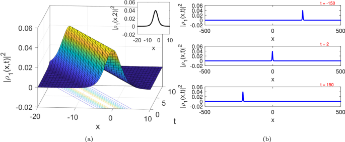
The bell-shape plots of \({{\left| {{\rho }_{1}}(x,t) \right| }^{2}}\), where \(\alpha = 1,w= -1,\eta _{2}=1,{\eta }_{1}=0.5,\kappa = 0.3,\) and \(u= -0.36\).
Fig. 2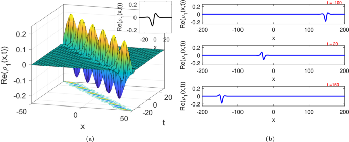
The mixed dark-bright plots of \(\operatorname {Re}({{\rho }_{1}}(x,t))\), where \(\alpha = 1,w= -1,\eta _{2}=1,{\eta }_{1}=0.5,\kappa = 0.3,\) and \(u= -0.36\).
Fig. 3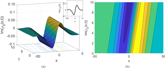
The dark-bright plots of \(\operatorname {Im}({{\rho }_{5}}(x,t))\), where \(\alpha = 1,w= 1.1,\eta _{3}=1,{\eta }_{1}=0.9,\kappa =0.1,\) and \(u= -0.1\).
Fig. 4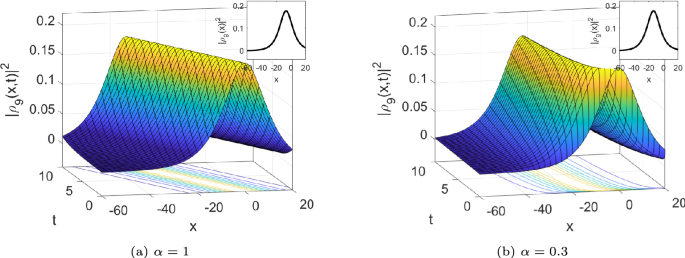
The comparison of bright plots of \(|{{\rho }_{9}}(x,t)|^2\) , where \(w=2,\eta _{3}=1,{\eta }_{2}=1,\kappa =-0.9,w=2\) and \(u= -0.1255\).
Result 1.
$$\begin{aligned} \begin{aligned}&\eta _{3}=-{\frac{4\,{w}^{2} \left( { r_{1}}\,{u}^{2}-{\kappa }^{2} \right) {\eta _{2}}^{2}+ \left( 4\,\eta _{1}\,{ r_{1}}\,{u}^{2}w-4\,\eta _{1}\,{\kappa }^{2}w-4\,\kappa \,{ r_{1}}\,{u}^{2} \right) \eta _{2}+ \left( { r_{1}}\,{u}^{2}-{\kappa }^{ 2} \right) {\eta _{1}}^{2} +\sqrt{{ K_{1}}}}{8{u}^{2} { r_{1}}\,\eta _{2}\, {\kappa }^{2}}},d_{0}=0,\\&d_{1}={\frac{\sqrt{\eta _{2}\,{ r_{2}}\, \left( -4\,{w}^{2} \left( { r_{1}}\,{u}^{2}+{\kappa }^{2} \right) {\eta _{2}}^{2}+ \left( -4\,\eta _{1}\,{ r_{1}}\,{u}^{2}w-4\,\eta _{1}\,{\kappa }^{2}w+4\, \kappa \,{ r_{1}}\,{u}^{2} \right) \eta _{2}+ \left( { r_{1}}\,{u}^{2}-{ \kappa }^{2} \right) {\eta _{1}}^{2} +\sqrt{{ K_{1}}} \right) }}{2\eta _{2}\,u{ r_{1}}\,p}}, \end{aligned} \end{aligned}$$
(15)
where
\(K_{1}=\left( 16\, \left( { r_{1}}\,{u}^{2}+{\kappa }^{2} \right) ^{2} \left( {w}^{2}{\eta _{2}}^{2}+\frac{{\eta _{1}}^{2}}{4}\right) +16\, \left( { r_{1}}\,{u}^{2}+{\kappa }^{2} \right) \left( \eta _{1}\,{ r_{1}}\,{u}^{2}w+ \eta _{1}\,{\kappa }^{2}w-2\,\kappa \,{ r_{1}}\,{u}^{2} \right) \eta _{2} \right) \left( \eta _{2}\,w+\frac{\eta _{1}}{2} \right) ^{2} .\)
From (5), (9), (12), (14), and 15, we can have the following optical soliton solution:
$$\begin{aligned} \begin{aligned}&\rho _{1}(x,t)=\frac{\sqrt{-\eta _{2}{(-4\,{w}^{2} \left( {\kappa }^{2}+{u}^{2} \right) {\eta _{2}}^{2}+ \left( -4 \,\eta _{1}\,{\kappa }^{2}w-4\,\eta _{1}\,{u}^{2}w+4\,\kappa \,{u}^{2} \right) \eta _{2}+{\eta _{1}}^{2}{u}^{2}-{\eta _{1}}^{2}{\kappa }^{2} )}+\sqrt{{ K_{2}}}}}{\eta _{2}u}\\&\,\operatorname {sech}(({-\frac{ \left( {\kappa }^{2}-{u}^{2} \right) \left( 4\,{w}^{2}{ \eta _{2}}^{2}+4\,w\eta _{1}\,\eta _{2}+{\eta _{1}}^{2} \right) +8\,\eta _{2}\,\kappa \,{u} ^{2}+\sqrt{{ K_{2}}}}{4\eta _{2}\,\kappa \,{u} \left( 2\,\eta _{2}\,w+\eta _{1} \right) }})\frac{t^{\alpha }}{\alpha })+x) \textrm{e}^{i ( -\kappa \,x+w\frac{t^{\alpha }}{\alpha } )}. \end{aligned} \end{aligned}$$
(16)
From (6), (9), (12), (14), and 15, we can have the following optical soliton solution:
$$\begin{aligned} \begin{aligned}&\rho _{2}(x,t)=\frac{\sqrt{\eta _{2}{(-4\,{w}^{2} \left( {\kappa }^{2}+{u}^{2} \right) {\eta _{2}}^{2}+ \left( -4 \,\eta _{1}\,{\kappa }^{2}w-4\,\eta _{1}\,{u}^{2}w+4\,\kappa \,{u}^{2} \right) \eta _{2}+{\eta _{1}}^{2}{u}^{2}-{\eta _{1}}^{2}{\kappa }^{2} )}+\sqrt{{ K_{2}}}}}{\eta _{2}u}\\&\,\operatorname {csch}(({-\frac{ \left( {\kappa }^{2}-{u}^{2} \right) \left( 4\,{w}^{2}{ \eta _{2}}^{2}+4\,w\eta _{1}\,\eta _{2}+{\eta _{1}}^{2} \right) +8\,\eta _{2}\,\kappa \,{u} ^{2}+\sqrt{{ K_{2}}}}{4\eta _{2}\,\kappa \,{u} \left( 2\,\eta _{2}\,w+\eta _{1} \right) }})\frac{t^{\alpha }}{\alpha })+x) \textrm{e}^{i ( -\kappa \,x+w\frac{t^{\alpha }}{\alpha } )}, \end{aligned} \end{aligned}$$
(17)
where
\(K_{2}=\left( 16\,\eta _{2}\, \left( {\kappa }^{2}+{u}^{2} \right) \left( \left( \eta _{2}\,w+\eta _{1} \right) \left( w{\kappa }^{2}+{u}^{2}w \right) -2\,\kappa \,{u}^{2} \right) +4\,{\eta _{1}}^{2} \left( u-\kappa \right) ^{ 2} \left( u+\kappa \right) ^{2} \right) \left( \eta _{2}\,w+\frac{\eta _{1}}{2} \right) ^{2}.\)
From (7), (9), (12), (14), and (15), we can have the following optical soliton solution:
$$\begin{aligned} \begin{aligned}&\rho _{3}(x,t)=-\frac{\sqrt{\eta _{2}{(-4\,{w}^{2} \left( {\kappa }^{2}+{u}^{2} \right) {\eta _{2}}^{2}+ \left( -4 \,\eta _{1}\,{\kappa }^{2}w-4\,\eta _{1}\,{u}^{2}w+4\,\kappa \,{u}^{2} \right) \eta _{2}-{\eta _{1}}^{2}{u}^{2}-{\eta _{1}}^{2}{\kappa }^{2} )}+\sqrt{{ K_{3}}}}}{\eta _{2}u}\\&\,\operatorname {sec}(({\frac{ \left( {\kappa }^{2}+{u}^{2} \right) \left( -4\,{w}^{2} {\eta _{2}}^{2}-4\,w\eta _{1}\,\eta _{2}-{\eta _{1}}^{2} \right) +4\,\eta _{2}\,\kappa \,{u }^{2}+\sqrt{{ K_{3}}}}{4\eta _{2}\,\kappa \,{u} \left( 2\,\eta _{2}\,w+\eta _{1} \right) }} )\frac{t^{\alpha }}{\alpha })+x) \textrm{e}^{i ( -\kappa \,x+w\frac{t^{\alpha }}{\alpha } )}. \end{aligned} \end{aligned}$$
(18)
From (8), (9), (12), (14), and (15), we can have the following optical soliton solution:
$$\begin{aligned} \begin{aligned}&\rho _{4}(x,t)=-\frac{\sqrt{\eta _{2}{(-4\,{w}^{2} \left( {\kappa }^{2}+{u}^{2} \right) {\eta _{2}}^{2}+ \left( -4 \,\eta _{1}\,{\kappa }^{2}w-4\,\eta _{1}\,{u}^{2}w+4\,\kappa \,{u}^{2} \right) \eta _{2}-{\eta _{1}}^{2}{u}^{2}-{\eta _{1}}^{2}{\kappa }^{2} )}+\sqrt{{ K_{3}}}}}{\eta _{2}u}\\&\,\operatorname {csc}(({\frac{ \left( {\kappa }^{2}+{u}^{2} \right) \left( -4\,{w}^{2} {\eta _{2}}^{2}-4\,w\eta _{1}\,\eta _{2}-{\eta _{1}}^{2} \right) +4\,\eta _{2}\,\kappa \,{u }^{2}+\sqrt{{ K_{3}}}}{4\eta _{2}\,\kappa \,{u} \left( 2\,\eta _{2}\,w+\eta _{1} \right) }} )\frac{t^{\alpha }}{\alpha })+x) \textrm{e}^{i ( -\kappa \,x+w\frac{t^{\alpha }}{\alpha } )}, \end{aligned} \end{aligned}$$
(19)
where
\(K_{3}=16\, \left( \eta _{2}\,w+\frac{\eta _{1}}{2} \right) ^{2} \left( \eta _{2}\, \left( u- \kappa \right) \left( \left( {w}^{2}\eta _{2}+\eta _{1}\,w-2\,\kappa \right) {u}^{2}-w \left( \eta _{2}\,w+\eta _{1} \right) {\kappa }^{2} \right) \left( u+\kappa \right) +\frac{{\eta 1}^{2} }{4}\left( {\kappa }^{2}+{u}^{2} \right) ^{2} \right) .\)
Result 2.
$$\begin{aligned} d_{0}=0,\eta _{2}=0,\kappa =\kappa ,w={\frac{\eta _{3}\,{ r_{1}}\,{u}^{2}-\eta _{3}\,{\kappa }^{2}+\kappa }{\eta _{1}}}, d_{1}={\frac{u\sqrt{-2\,\eta _{3}\,{ r_{2}}}}{p}}. \end{aligned}$$
(20)
Fig. 5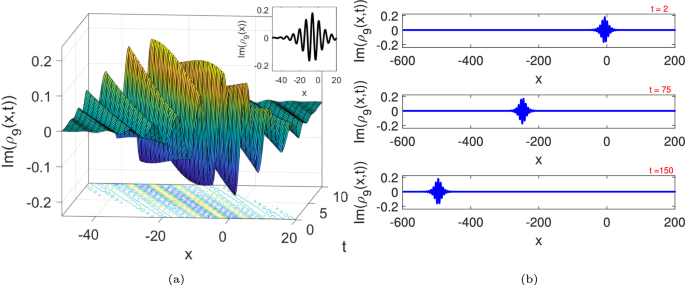
The mixed dark-bright plots of \(\operatorname {Im}({{\rho }_{9}}(x,t))\), where \(w=2,\eta _{3}=1,{\eta }_{2}=1,\kappa =-0.9,w=2,u= – 0.1255\) and \(t=2\).
Fig. 6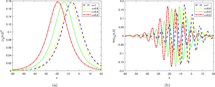
The 2D plots of \({{\left| {{\rho }_{9}}(x,t) \right| }^{2}}\) and \(\operatorname {Im}({{\rho }_{9}}(x,t))\), where \(w=2,\eta _{3}=1,{\eta }_{2}=1,\kappa =-0.9,w=2,u= -0.1255\) and \(t=2\).
From (5), (9), (12), (14), and (20) , we can have the following optical soliton solution:
$$\begin{aligned} \begin{aligned}&\rho _{5}(x,t)=\sqrt{2\eta _{3}} u \textrm{sech} \left( u \left( x +{\frac{ \left( 2\, \eta _{3}\,\kappa -1 \right) {t}^{\alpha }}{\alpha \,\eta _{1}}} \right) \right) {\textrm{e}^{i \left( -\kappa \,x+{\frac{ \left( -\eta _{3}\,{\kappa }^ {2}+\eta _{3}\,{u}^{2}+\kappa \right) {t}^{\alpha }}{\alpha \,\eta _{1}}} \right) }}. \end{aligned} \end{aligned}$$
(21)
From (6), (9), (12), (14), and (20) , we can have the following optical soliton solution:
$$\begin{aligned} \begin{aligned}&\rho _{6}(x,t)=\sqrt{-2\eta 3} u \textrm{csch} \left( u \left( x +{\frac{ \left( 2\, \eta _{3}\,\kappa -1 \right) {t}^{\alpha }}{\alpha \,\eta _{1}}} \right) \right) {\textrm{e}^{i \left( -\kappa \,x+{\frac{ \left( -\eta _{3}\,{\kappa }^ {2}+\eta _{3}\,{u}^{2}+\kappa \right) {t}^{\alpha }}{\alpha \,\eta _{1}}} \right) }}. \end{aligned} \end{aligned}$$
(22)
From (7), (9), (12), (14), and (20) , we can have the following optical soliton solution:
$$\begin{aligned} \begin{aligned}&\rho _{7}(x,t)=\sqrt{-2\eta _{3}} u \textrm{sec} \left( u \left( x +{\frac{ \left( 2\, \eta _{3}\,\kappa -1 \right) {t}^{\alpha }}{\alpha \,\eta _{1}}} \right) \right) {\textrm{e}^{i \left( -\kappa \,x+{\frac{ \left( -\eta _{3}\,{\kappa }^ {2}-\eta _{3}\,{u}^{2}+\kappa \right) {t}^{\alpha }}{\alpha \,\eta _{1}}} \right) }}. \end{aligned} \end{aligned}$$
(23)
From (8), (9), (12), (14), and (20) , we can have the following optical soliton solution:
$$\begin{aligned} \begin{aligned}&\rho _{8}(x,t)=\sqrt{-2\eta 3} u \textrm{csc} \left( u \left( x +{\frac{ \left( 2\, \eta _{3}\,\kappa -1 \right) {t}^{\alpha }}{\alpha \,\eta _{1}}} \right) \right) {\textrm{e}^{i \left( -\kappa \,x+{\frac{ \left( -\eta _{3}\,{\kappa }^ {2}-\eta _{3}\,{u}^{2}+\kappa \right) {t}^{\alpha }}{\alpha \,\eta _{1}}} \right) }}. \end{aligned} \end{aligned}$$
(24)
Result 3
$$\begin{aligned} d_{0}=0,\eta _{2}=0, d_{1}={\frac{\sqrt{-2\,\eta _{3}\,{ r_{2}}}u}{p}}, \eta _{1}={\frac{ \left( { r_{1}}\,{u}^{2}-{\kappa }^{2} \right) \eta _{3}+\kappa }{w }}. \end{aligned}$$
(25)
From (5), (9), (12), (14), and (25) , we can have the following optical soliton solution:
$$\begin{aligned} \begin{aligned}&\rho _{9}(x,t)=\sqrt{2\eta _{3}}u\textrm{sech} \left( u \left( x+{\frac{ \left( 2\, \eta _{3}\,\kappa -1 \right) w{t}^{\alpha }}{\alpha \, \left( \left( -{ \kappa }^{2}+{u}^{2} \right) \eta _{3}+\kappa \right) }} \right) \right) \textrm{e}^{i ( -\kappa \,x+{\frac{w{t}^{\alpha }}{\alpha }} ) }. \end{aligned} \end{aligned}$$
(26)
From (6), (9), (12), (14), and (25), we can have the following optical soliton solution:
$$\begin{aligned} \begin{aligned}&\rho _{10}(x,t)=\sqrt{-2\eta _{3}}u\textrm{csch} \left( u \left( x+{\frac{ \left( 2\, \eta _{3}\,\kappa -1 \right) w{t}^{\alpha }}{\alpha \, \left( \left( -{ \kappa }^{2}+{u}^{2} \right) \eta _{3}+\kappa \right) }} \right) \right) \textrm{e}^{i ( -\kappa \,x+{\frac{w{t}^{\alpha }}{\alpha }} ) }.\\ \end{aligned} \end{aligned}$$
(27)
From (7), (9), (12), (14), and (25), we can have the following optical soliton solution:
$$\begin{aligned} \begin{aligned}&\rho _{11}(x,t)=\sqrt{-2\eta _{3}}u\textrm{sec} \left( u \left( x+{\frac{ \left( 2\, \eta _{3}\,\kappa -1 \right) w{t}^{\alpha }}{\alpha \, \left( \left( -{ \kappa }^{2}-{u}^{2} \right) \eta _{3}+\kappa \right) }} \right) \right) \textrm{e}^{i ( -\kappa \,x+{\frac{w{t}^{\alpha }}{\alpha }} ) }.\\ \end{aligned} \end{aligned}$$
(28)
From (8), (9), (12), (14), and (25), we can have the following optical soliton solution:
$$\begin{aligned} \begin{aligned}&\rho _{12}(x,t)=\sqrt{-2\eta _{3}}u\textrm{csc} \left( u \left( x+{\frac{ \left( 2\, \eta _{3}\,\kappa -1 \right) w{t}^{\alpha }}{\alpha \, \left( \left( -{ \kappa }^{2}-{u}^{2} \right) \eta _{3}+\kappa \right) }} \right) \right) \textrm{e}^{i ( -\kappa \,x+{\frac{w{t}^{\alpha }}{\alpha }} ) }.\\ \end{aligned} \end{aligned}$$
(29)
Fig. 7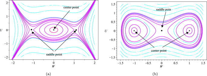
Phase portraits of the system’s bifurcations are depicted under different conditions for \(\mu _{1}\) and \(\mu _{2}\), using various parameter values for Case 5.1 and Case 5.2.
Fig. 8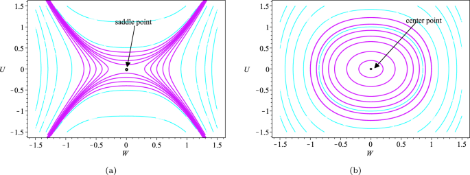
Phase portraits of the system’s bifurcations are depicted under different conditions for \(\mu _{1}\) and \(\mu _{2}\), using various parameter values for Case 5.3 and Case 5.4.