Device
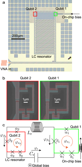
Figure 1a shows an optical microscopy image of the artificial-atom–resonator circuit. The LC resonator is composed of an interdigital capacitor and a line inductor made of a superconducting thin film33,34. The two flux qubits are inductively coupled to the LC resonator via a Josephson junction (Fig. 1b), which increases the strength of couplings to the ultrastrong regime. Small dots around the two qubits are flux traps that prevent vortex fluctuations during the measurements35. The energies of the flux qubits36 can be changed by applying an external magnetic flux to the loop from a global coil and using an on-chip bias line. Figure 1c shows the equivalent circuit with lumped elements and Josephson junctions.
Fig. 1: Device.
a Optical microscopy image of the measured sample. The sample holder has a coil to bias a uniform magnetic field from the back surface of the chip. Qubit 1 has a local bias line that changes the magnetic flux of the qubit loop. The spectrum is measured using a vector network analyzer (VNA) for probing and reading from the transmission line shown below the circuit. b False-color SEM images of qubits 1 and 2. The design parameters of both qubit junctions are the same. Different colors represent different layers of aluminum deposited via double-angle shadow evaporation. c Equivalent circuit diagram of the sample. The symbols αi, βi, ai, and bi (i ∈ {1, 2}) label each Josephson junction, while φ denotes the phase difference across a circuit component.
The Hamiltonian of the entire system is37,38,39
$${\hat{{{{\mathcal{H}}}}}}_{{{{\rm{tot}}}}}={\hat{{{{\mathcal{H}}}}}}_{{{{\rm{q1}}}}}+{\hat{{{{\mathcal{H}}}}}}_{{{{\rm{q2}}}}}+{\hat{{{{\mathcal{H}}}}}}_{{{{\rm{r}}}}}+{\hat{{{{\mathcal{H}}}}}}_{{{{\rm{int}}}}}\,,$$
(1)
where \({\hat{{{{\mathcal{H}}}}}}_{{{{\rm{q}}}}k}\) (k = 1, 2), \({\hat{{{{\mathcal{H}}}}}}_{{{{\rm{r}}}}}\), and \({\hat{{{{\mathcal{H}}}}}}_{{{{\rm{int}}}}}\) represent the qubits, resonator, and atom–resonator plus atom–atom couplings, respectively. The Hamiltonian of the resonator is \({\hat{{{{\mathcal{H}}}}}}_{{{{\rm{r}}}}}=\hslash {\omega }_{{{{\rm{r}}}}}({\hat{a}}^{{{\dagger}} }\hat{a}+1/2)\), where \({\omega }_{{{{\rm{r}}}}}\equiv 1/\sqrt{{L}_{{{{\rm{r}}}}}{C}_{{{{\rm{r}}}}}}\) is the resonance frequency, \(\hat{a}\equiv ({\hat{\phi }}_{{{{\rm{r}}}}}-i{Z}_{{{{\rm{r}}}}}{\hat{q}}_{{{{\rm{r}}}}})/\sqrt{2\hslash {Z}_{{{{\rm{r}}}}}}\) is the annihilation operator, \({Z}_{{{{\rm{r}}}}}=\sqrt{{L}_{{{{\rm{r}}}}}/{C}_{{{{\rm{r}}}}}}\) is the characteristic impedance of the LC resonator, and \({\hat{q}}_{{{{\rm{r}}}}}\) is the conjugate variable of \({\hat{\phi }}_{{{{\rm{r}}}}}={\Phi }_{0}{\hat{\varphi }}_{{{{\rm{r}}}}}\). Here, Φ0 is the flux quantum and the flux φr is defined in Fig. 1c. The Hamiltonian of the k-th artificial atom is
$${\hat{{{{\mathcal{H}}}}}}_{{{{\rm{q}}}}k}\equiv 4{E}_{{{{\rm{c}}}}k}{\hat{{{{\bf{q}}}}}}_{k}^{{{{\rm{T}}}}}{{{{\bf{M}}}}}_{k}^{-1}{\hat{{{{\bf{q}}}}}}_{k}+{E}_{{{{\rm{Lr}}}}}{\hat{\varphi }}_{\beta k}^{2}+{\hat{{{{\mathcal{U}}}}}}_{{{{\rm{J}}}}k}\,,$$
(2)
where Eck is the charging energy of the Josephson junction ak (see Fig. 1b and 1c), φβk represents the phase differences in each β-junction of qubits, Mk is the normalized mass matrix, \({E}_{{{{\rm{Lr}}}}}={\Phi }_{0}^{2}/(2{L}_{{{{\rm{r}}}}})\), and \({\hat{{{{\mathcal{U}}}}}}_{{{{\rm{J}}}}k}\) is the qubit potential energy of Josephson junctions:
$$\begin{array}{rc} \,\,{\hat{{{{\mathcal{U}}}}}}_{{{{\rm{J}}}}k}({\hat{\varphi }}_{{{{\rm{e}}}}k})=& -\,{E}_{{{{\rm{J}}}}k}\,\left[\,{\beta }_{k}\cos ({\hat{\varphi }}_{\beta k})\,+\,\cos ({\hat{\varphi }}_{ak})\,+\,\cos ({\hat{\varphi }}_{bk})\right.\\ &\left.+{\alpha }_{k}\cos ({\varphi }_{{{{\rm{e}}}}k}-{\hat{\varphi }}_{ak}-{\hat{\varphi }}_{bk}-{\hat{\varphi }}_{\beta k})\right]\,.\end{array}$$
(3)
Here, EJk is the current energy of the Josephson junction ak, φik (i = α, a, b) are the phase differences in each junction αk, ak, and bk, and φek represents the external flux for the loop of each atom. The interaction Hamiltonian
$${\hat{{{{\mathcal{H}}}}}}_{{{{\rm{int}}}}}=-{E}_{{{{\rm{Lr}}}}}({\hat{\varphi }}_{\beta 1}{\hat{\varphi }}_{{{{\rm{r}}}}}-{\hat{\varphi }}_{\beta 2}{\hat{\varphi }}_{{{{\rm{r}}}}}+{\hat{\varphi }}_{\beta 1}{\hat{\varphi }}_{\beta 2})$$
(4)
is obtained from the boundary condition (Kirchhoff’s voltage law) of the loop forming the resonator with the elements Lr and Cr.
By approximating each atom as a two-level system40 on the basis of persistent currents of the superconducting loop, we obtain the total Hamiltonian in Eq. (1) as
$${\hat{{{{\mathcal{H}}}}}}_{{{{\rm{tot}}}}}/\hslash \simeq \,\,{\omega }_{{{{\rm{r}}}}}{\hat{a}}^{{{\dagger}} }\hat{a}\,+\,\frac{{\varepsilon }_{1}}{2}{\hat{\sigma }}_{z1}\,+\,\frac{{\Delta }_{1}}{2}{\hat{\sigma }}_{x1}\,+\,\frac{{\varepsilon }_{2}}{2}{\hat{\sigma }}_{z2}\,+\,\frac{{\Delta }_{2}}{2}{\hat{\sigma }}_{x2}\\ -({g}_{1}{\hat{\sigma }}_{z1}-{g}_{2}{\hat{\sigma }}_{z2})({\hat{a}}^{{{\dagger}} }+\hat{a})-\frac{2{g}_{1}{g}_{2}}{{\omega }_{{{{\rm{r}}}}}}{\hat{\sigma }}_{z1}{\hat{\sigma }}_{z2}\,,$$
(5)
where εk is the persistent current energy of each qubit, Δk is the qubit energy gap when εk = 0, while \({\hat{\sigma }}_{zk}\) and \({\hat{\sigma }}_{xk}\) are the Pauli matrices for the k-th qubit. We define εk > 0 when the qubit current flows anticlockwise and vice versa.
After a unitary transformation that diagonalizes the atomic Hamiltonians \({\hat{{{{\mathcal{H}}}}}}_{{{{\rm{qk}}}}}\), we obtain a generalized Dicke Hamiltonian41 with spin–spin interaction:
$${\hat{{{{\mathcal{H}}}}}}_{{{{\rm{tot}}}}}/\hslash \simeq \,\,{\omega }_{{{{\rm{r}}}}}{\hat{a}}^{{{\dagger}} }\hat{a}+\frac{{\omega }_{{{{\rm{q1}}}}}}{2}{\hat{\sigma }}_{z1}+\frac{{\omega }_{{{{\rm{q2}}}}}}{2}{\hat{\sigma }}_{z2}\\ -({g}_{1}{\hat{{{\Lambda }}}}_{1}-{g}_{2}{\hat{{{\Lambda }}}}_{2})({\hat{a}}^{{{\dagger}} }+\hat{a})-\frac{2{g}_{1}{g}_{2}}{{\omega }_{{{{\rm{r}}}}}}{\hat{{{\Lambda }}}}_{1}{\hat{{{\Lambda }}}}_{2}\,,$$
(6)
where \({\omega }_{{{{\rm{q}}}}k}={{{\rm{sgn}}}}({\varepsilon }_{k}){({\varepsilon }_{k}^{2}+{\Delta }_{k}^{2})}^{1/2}\) is the qubit frequency and \({\hat{{{\Lambda }}}}_{k}=(\cos {\theta }_{k}\,{\hat{\sigma }}_{xk}+\sin {\theta }_{k}\,{\hat{\sigma }}_{zk})\) gives the direction of the interaction, with \({\theta }_{k}\simeq -\arctan ({\varepsilon }_{k}/{\Delta }_{k})\) (see Methods for more details). For θk = 0 (εk = 0), the interaction is purely transverse. When θk ≠ 0, the interaction has a longitudinal component and the one–photon–exciting–two–atoms effect is allowed.
Energy spectrum
Figure 2a shows the raw data of the measured spectrum as a function of the persistent current energy ε1 of qubit 1, which are obtained after fixing the value of ε2/2π at −3.22 GHz when ε1 = 0. In Fig. 2b, the spectrum is fitted with the numerically calculated transition frequencies ωij between the i-th and j-th eigenstates of the total Hamiltonian \({\hat{{{{\mathcal{H}}}}}}_{{{{\rm{tot}}}}}\). The persistent current energy for qubit 2 and the resonator frequency are affected by the external magnetic flux applied to qubit 18. Thus, to derive the transition frequencies ωij, we substitute ε2 → ε2 + Aε1 and ωr → ωr(1 + B±ε1) in Eq. (5), where A and B± are small fitting parameters listed in Table 1. We use two different values for B± because the spectrum is asymmetric with respect to the sign of ε1, i.e., B+ is used when ε1≥0 and vice versa. Including A and B±, we use 11 parameters in total for the fit. These also include the bias current offset Ib0, when ε1 = 0, and the persistent current coefficient \({\tilde{\varepsilon }}_{0}\) to derive \(\hslash {\varepsilon }_{1}={I}_{{{{\rm{p}}}}}{\Phi }_{0}({\varphi }_{{{{\rm{e1}}}}}-0.5)=\hslash {\tilde{\varepsilon }}_{0}({I}_{{{{\rm{b}}}}}-{I}_{b0})\), where Ip is the persistent current of qubit 1, and Ib is the bias current from the room-temperature current source. We use a photo-processing technique to obtain peak points from the spectrum37,42,43 and the quantum toolbox in Python for numerical calculations44,45.
Fig. 2: Transmission spectra.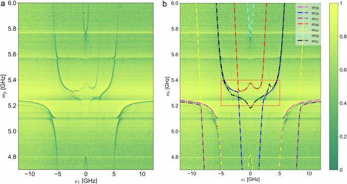
Pump frequency ωp from the vector network analyzer versus the persistent current energy ε1 of qubit 1. a Raw data of the observed single-tone spectrum of the sample shown in Fig. 1. b Observed single-tone spectrum with fitted curves corresponding to the state transition frequencies ωij between the i-th and j-th eigenstates of Hamiltonian (6). The fit parameters are g1/2π = 3.33, g2/2π = 3.45, Δ1/2π = 1.31, Δ2/2π = 1.27, ωr/2π = 5.15, and ε2/2π = −3.22 GHz. At around ωp/2π = 5.09 GHz and 5.57 GHz, parasitic modes can be seen, which originate from, for example, sample ground planes and/or the measurement environment, which includes the sample holder and microwave components coupled to the system.
Table 1 List of the fitting parameters used in Figs. 2 and 3
Flux qubits 1 and 2 are almost identical except for the loop size; consequently, they have similar fitting parameters; i.e., Δq1 ≃ Δq2 ≃ 0.25 ωr. We find atom-resonator coupling rates of g1/ωr = 0.67 and g2/ωr = 0.69, indicating that the artificial atoms are ultrastrongly coupled with the resonator.
One photon simultaneously excites two atoms
We indicate with \(\left\vert {\psi }_{i}\right\rangle\) the eigenstate of the system Hamiltonian \({\hat{{{{\mathcal{H}}}}}}_{{{{\rm{tot}}}}}\) with eigenenergies ℏωi0. The \({\omega }_{{{{\rm{q}}}}i}{\hat{\sigma }}_{zi}/2\) terms in Eq. (6) define the ground \(\left\vert g\right\rangle\) and excited \(\left\vert e\right\rangle\) atomic bare states.
In Fig. 3a, which is an enlarged view of the red dashed rectangle in Fig. 2b, the black arrow indicates the anticrossing between the eigenstates \(\left\vert {\psi }_{3}\right\rangle\) and \(\left\vert {\psi }_{4}\right\rangle\) (see Fig. 3b), with eigenfrequencies ω30 and ω40. In agreement with this anticrossing, Fig. 3c shows the numerically calculated projection \({P}_{j}^{(i)}\equiv {| \left\langle {\psi }_{i}| j\right\rangle | }^{2}\) of the third and fourth eigenstates \(\left\vert {\psi }_{i}\right\rangle \,(i=3,4)\) on the bare states \(\left\vert j\right\rangle=\{\left\vert gg1\right\rangle,\left\vert ee0\right\rangle \}\) as a function of ε1. Here, it is possible to see that the third and fourth eigenstates are the approximate symmetric and antisymmetric superpositions of \(\left\vert gg1\right\rangle\) and \(\left\vert ee0\right\rangle\), respectively. Considering also that the sum of the dressed qubit frequencies is nearly equal to the dressed resonator frequency, the anticrossing is the signature of the one–photon–exciting–two–atoms effect (see Methods for more details). Half of the minimum split between ω30 and ω40 in the spectrum gives the effective coupling between \(\left\vert gg1\right\rangle\) and \(\left\vert ee0\right\rangle\), that is 22.8 MHz (see Supplementary Information).
Fig. 3: Anticross between \(\left\vert gg1\right\rangle\) and \(\left\vert ee0\right\rangle\).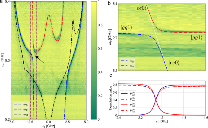
a Enlarged view of the central part of the spectrum in Fig. 2b with fitting curve. The fitting reproduces the spectrum well. b Enlarged image of the anticrossing between ω30 and ω40. The white lines represent the eigenmodes of \(\left\vert gg1\right\rangle\) and \(\left\vert ee0\right\rangle\) in the non-interacting Hamiltonian (see Methods for more details). c Projection of the third and fourth eigenstates calculated using Hamiltonian in Eq. (6) with the fitting parameters to the bare states \(\left\vert gg1\right\rangle\) and \(\left\vert ee0\right\rangle\).
With respect to the theoretical prediction in ref. 28 (g/ωr ≃ 0.1–0.2), our system has a much larger coupling (g/ωr ≃ 0.7). This implies that the system eigenstates should have a strong dressing, and in principle we could not observe a clean “one–photon–exciting–two–atoms” effect. On the contrary, Fig. 3c shows that the dressing is low for those states, and, as shown in Fig. 5, our system can still be considered formed by two separated two-level atoms and one cavity mode with shifted eigenfrequencies. This behavior is heuristically justified by the fact that spin–spin and spins–light couplings are competing interactions and that the longitudinal interaction “decouples” for specific values of the signs of ε1 and ε2. The signature of this “longitudinal decoupling” is given by the asymmetry in the spectrum with respect to the sign of ε1. Assuming that there are only longitudinal couplings, in the interaction part of Eq. (6), the operator \(({\hat{a}}^{{{\dagger}} }+\hat{a})\) should generate coherent states of light in the ultrastrong coupling regime46. However, considering ε1 ε2 M = m1 − m2 = 0, where mk = ± 1 is the eigenstate of \({\hat{\sigma }}_{zk}\,(k=1,2)\) (see Methods for more details). As a result, the ground \(\left\vert gg\right\rangle\) and excited \(\left\vert ee\right\rangle\) states, which have M = 0, have no coherent states associated with them. Nevertheless, the transverse interactions still affect our system, generating a small dressing that reduces the projections \({P}_{gg1}^{(4)}\) and \({P}_{ee0}^{(3)}\) to almost 0.8 at ε1/2π = −2.4 GHz.