Quantitative models of resistance evolution
We developed mathematical models of resistance evolution that described the response of a population of cancer cells to periodic drug treatment. We aimed to infer the dynamics solely using the change in total population size and relatedness between surviving cell lineages. As such, we modelled the evolution of phenotypes within a cell population that controls the response to treatment and the transitions between these phenotypes. Our approach was to begin with simple models of resistance evolution and add additional complexity only when simple models failed to explain data. We designed three models of increasing complexity that encompass behaviours previously observed during the emergence of cancer cell resistance. Full model details are provided in Supplementary Note 1.
Model A: the first and simplest model (which we coin ‘unidirectional transitions’) consists of two phenotypes: sensitive and resistant. A ‘pre-existing resistance fraction’ parameter (ρ) controls the initial conditions of the model by setting the proportion of cells with the resistant phenotype when the model begins (t0). Cells can divide with phenotype-specific birth and death rates (sensitive: bS,dS and resistant: bR,dR). A ‘cost’ parameter (δ) controls a fitness penalty associated with the resistant phenotype in the untreated environment. Including a fitness penalty allows us to test the assumption that, in the absence of treatment, resistant cells exhibit a reduced net growth rate relative to sensitive cells: this behaviour has been observed in experimentally generated resistant cancer cell lines17 and is significant for phenomena including the existence of slowly dividing ‘persister’ cells18 and drug ‘addiction’ whereby resistant cells fail to grow in the absence of treatment19. Fitness penalties associated with a resistant phenotype also influence tumour containment strategies20. A switching parameter (μ) controls the probability of cells transitioning from the sensitive to resistant phenotype per cell division.
Therapy was modelled by modifying the death rate of cells. For sensitive cells, the death rate increases as a function of D(t), with D(t) representing the effective drug concentration at time t. Omitting the pharmacokinetics of the drug treatment would impair the model’s ability to recover observed changes in cell population sizes, as the cytotoxic effects of a drug are not realised immediately. We assume a pharmacokinetic model where the focus is on the change in the realised effect of the drug on cells, rather than directly modelling the drug concentration. The parameters Dc and κ regulate the strength and rate of accumulation/reduction of this effect, respectively. This model does not distinguish between intrinsic and extrinsic cellular factors; for instance, the increasing cytotoxicity experienced by cells following the addition of treatment could be affected by the drug’s chemistry, cellular efflux mechanisms, or some combination of the two. Furthermore, we make no assumption concerning the specific molecular change or mechanism that controls resistance in our models and instead focus on the phenotypes as dictating the probability of survival during treatment. The parameter ψ models the survival probability of the resistant cells under treatment: ψ = 1.0 denotes complete resistance, whereas when ψ = 0.0 the sensitive and resistant cells experience the same level of drug-induced death.
To summarise, in this model the total cell population’s response to treatment is a product of the proportion of resistance (dictated by ρ, δ and μ), the effective strength of the drug at a given time (dictated by Dc and κ) and the strength of the resistant phenotype (dictated by ψ).
Model A allowed us to explore some simpler evolutionary scenarios of interest: compared to sensitive cells, resistant cells can either be absent or pre-exist at varying frequencies (by varying ρ), be either strongly or weakly resistant (by varying ψ) and can potentially grow at slower rates relative to sensitive cells in the untreated environment (by varying δ). Additionally, phenotypic switching from sensitive to resistant (μ) can vary, with lower probabilities representing the dynamics of genetic mutations and higher probabilities representing rapid non-genetic phenomena. Importantly, we did not define a strict boundary between these two possibilities, and instead can only reject genetic mutations when transitions occur at rates that are too high to be biologically feasible.
We considered which behaviours relevant to cancer resistance evolution model A (‘unidirectional switching’) could not reproduce. There are multiple reports of reversible transitions between resistant and sensitive phenotypes21, or the emergence of faster growing resistant cells from a slow cycling, drug tolerant population in response to the commencement of treatment11. We therefore developed more complex models that could capture these dynamics.
Model B: ‘bidirectional transitions’ includes an additional behaviour whereby resistant cells can transition back to the sensitive phenotype with an independent probability (σ) per cell division. Previously, we had assumed resistance phenotypes arose unidirectionally (i.e., a resistant cell could not transition back to being sensitive). This modification allowed behaviours reminiscent of rapid, reversible, non-genetic transitions between phenotypes at higher probabilities, or forward and back mutations at lower probabilities.
Model C: ‘escape transitions’ incorporates an additional phenotype we label ‘escape’. These cells behave like resistant cells in Models A and B but lack the fitness cost. As in model B, resistant cells can transition back to sensitive cells (with probability σ). However, resistant cells also now have a chance of transitioning to the escaped phenotype with a maximum probability of α per division. The transitions from resistant to escaped are scaled by a function of the current drug concentration (α · f D(t)) and are therefore only possible once treatment begins, permitting behaviours that resemble observations where transition rates and resistant phenotypes emerge in a drug-dependent manner22,23. Given transitions to the escape cells cannot commence until treatment begins, the initial conditions are still determined by the pre-existing resistance fraction parameter (ρ). With this modification the model can generate behaviours where the commencement of treatment allows slower growing cells (‘resistant cells’ in all three of our models) to transition to a faster growing phenotype also refractory to treatment (‘escape’ in model C).
Modelling Experimental Evolution: In all models, we coded-in features that enabled direct comparison to an empirical in vitro evolution experiment: the ability to track the lineage identity of cells uniquely labelled when the experiment commences (‘in silico’ lineage tracing); a mutual expansion period before splitting cells into replicate sub-populations (where an initial barcoded pool of cells was split into replicate populations that were then independently evolved in parallel); exposing sub-populations to periodic drug treatment; and population sampling bottlenecks of known magnitude at given times. Our different models of resistance evolution—Models A,B,C—control the phenotypic composition of the cell populations during these sampling bottlenecks. The initial conditions (ρ) correspond to the composition of phenotypes when the simulations begin with N0 cells, when cells are also assigned a unique lineage identity (an ‘in silico’ barcode) (Fig. 1). Cells from an expanded population (Nexp) were sampled without replacement and allocated to drug-treatment replicates (DTx, where x = 1, 2, 3, 4). Additional sampling simulates the ‘passaging’ steps of evolution experiments (where P1 = Passage 1, etc.). Due to the limitation on population size imposed by the volume of tissue culture vessels in vitro, growth in all models was modelled as logistic growth with a fixed carrying capacity, C (see Supplementary Note 1) with a constant value guided by the empirical data. Cell populations were grown until a maximum population size (Nmax) was reached (where Nmax 24,25.
Fig. 1: Overview of the experimental simulation and sampling procedure used to generate synthetic data.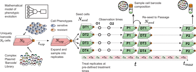
Unknown parameters govern the behaviour of cell phenotypes and their response to treatment. Fixed parameters control key experimental steps, including the initial number of uniquely barcoded cells, their expansion time, sampling bottlenecks when splitting into experimental replicates, and the timing of treatment windows. The drug-treatment replicates (DT1-4), population size observation timepoints (O1,2) and passages (P1-2) shown correspond to the experimental design used in our simulation modelling results.
We compare our models to existing mathematical models of phenotypic evolution in cancer. Model A shares features with commonly employed models of resistance evolution, incorporating two phenotypic compartments (sensitive and resistant), different pre-existing fractions of resistance, phenotype-specific birth and death rates26,27,28 and modifications to these rates based on the current effective drug concentration29,30,31. Many studies allow for transitions from sensitive to resistant phenotypes, although this is often assumed to occur at a low probability, with values chosen based on estimates of mutation rates in cancer cells32. While many models assume binary treated or untreated environments, fewer have directly incorporated drug pharmacokinetics to modify birth and death rates in a concentration-dependent manner (although see: Johnson et al.33; Poels et al.34).
Model B is comparable to previous theoretical work investigating how stochastic phenotypic switching can promote survival in bacteria35,36. These behaviours have also been modelled in cancer, where common features mirroring our own include asymmetrical transitions between phenotypes at probabilities too high to occur via genetic mutations37,38. Importantly, we use our models to infer non-genetic phenotypic transitions by using these high probabilities to exclude genetic mutations. This ‘population-down’ approach contrasts with modelling strategies that predict non-genetic phenotypic transitions as a property of gene regulatory networks39,40.
Model C, our most complex model with three phenotypes, permits unidirectional transitions to a third phenotype, ‘escape,’ as a function of the current effective drug treatment (α⋅fD(t)), mirroring previous models that include drug-induced transitions from sensitivity to resistance11,22,41 and epigenetic rewiring to a stably resistant state that is drug-dependent and non-reversible42.
In contrast to many existing models, we aim to infer multiple behaviours relevant to both drug treatment and resistance evolution from the data simultaneously, including the rate of change (κ), the strength of selection exerted by the drug (Dc), and the magnitude of resistance (ψ). Our modelling also explicitly accounts for the technical sampling steps encountered during long-term resistance evolution experiments which are particularly relevant in lineage tracing setups8,43.
Population and lineage distributions during treatment are determined by phenotype behaviours
We explored the population dynamics during treatment quantitatively using our modelling framework. We performed simulations with biologically feasible parameter values and recorded how replicate sub-populations responded to rounds of treatment. We hypothesised that phenotypic behaviours of interest—for example, transition rates between sensitive and resistant states and the proportion of resistance when treatment commences—could be inferred from empirical measurements. Each of our models was simulated to generate data that would typically be measured during a long-term evolution experiment. Per simulation, we modelled four drug-treatment replicates (DT1-4). These replicate cell populations had been sampled from the same expanded population or cells that had been uniquely labelled with in silico lineage tags – ‘barcodes’—when the simulation began. Given a sufficient expansion period, closely related cells that share a lineage barcode should be present in multiple replicates. We also saved the total population size at two ‘observation’ timepoints (O1,O2) and each Passage step (P1,P2). We reasoned that comparing the change in total population size and the lineage identify of surviving subclones within and between replicates could be used to distinguish different evolutionary scenarios of interest.
Initially we focussed on the change in the total number of cells over time.
We found that changes in total cell population sizes during treatment are driven by the proportion of each phenotype and their response to treatment.
In model A, unsurprisingly, when resistance was initially more common (higher values of ρ), the time until the maximum population size was reached was shorter (Fig. 2A, B). Interestingly, even in cases where resistance was initially rare or absent, the changes in total cell population sizes between replicates can be highly repeatable (Fig. 2B): despite the bottleneck exerted by treatment, the similar proportions of resistance in each replicate generated by transitions to resistance (μ) and the shared survival probability during treatment (ψ) generate consistent growth dynamics.
Fig. 2: Quantitative models of resistance evolution exhibit distinct cell population dynamics during treatment.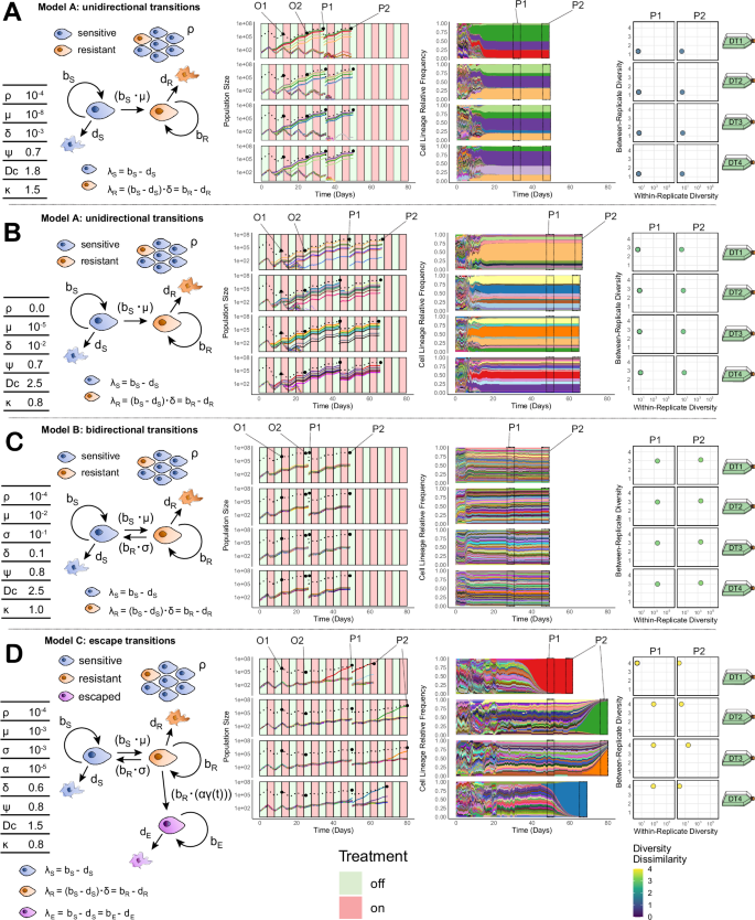
A–D Per panel: (Left) Schematics of different evolutionary models, highlighting key parameters that control the behaviour of resistant, sensitive, and escape phenotypes (see text and Supplementary Note 1 for full descriptions). (Middle) Total cell population size trajectories (dashed lines) and the top 20 lineage population sizes (coloured lines)/relative frequencies (shaded areas) across four experimental drug-treatment replicates (DT1-4, rows). Lineage colours are consistent between replicates per panel. Four total cell size observations per replicate (two intermediate population size timepoints (O1 & O2) and two passage size timepoints (P1 & P2)) are highlighted. (Right) Lineage diversity statistics for the 4 drug-treatment replicates at two passage timepoints (P1 & P2 – columns), including within- replicate lineage (x-axis) and between-replicate diversity (y-axis). Simulation parameters: bx—birth rate of phenotype x, dX—death rate of phenotype x, ρ—pre-existing fraction of resistance, μ—sensitive to resistant transition probability per cell division, σ —resistant to sensitive transition probability per cell division, α—resistant to escape transition probability per cell division, γ—normalised effective drug concentration, ψ—strength of the resistant phenotype, Dc— maximum strength of the drug, κ—accumulation/decay rate of the drug. Source data including the full list of parameters used for the simulations are provided as a Source Data file.
In all models, if the effective phenotype transition probabilities were very low, the differing lag times preceding the emergence of treatment refractory populations could produce stochasticity in the time taken for the population to recover. This was especially true in model C (‘escape transitions’) when the transition from ‘resistant’ to ‘escape’ (α) was low: a population of slower growing resistant cells survive initial rounds of treatment before rarer transitions to the faster growing escape phenotype emerge during treatment (Fig. 1D).
We next considered the signal in the lineage distributions (clone size distributions) over time. Phenotypic transitions alter the relationship between phenotype and the lineage identity assigned at the beginning of the experiment. When transitions are rare, lineage identity mirrors phenotype identity, but this correlation is progressively lost at higher phenotypic transition rates. Combined with the known sampling bottlenecks and other evolutionary parameters controlling the phenotype-specific growth rates and strength of selection exerted by treatment, these behaviours determine the identify of surviving lineages.
Current empirical lineage tracing systems enable tracking of over 106 unique lineages. The sampling design we explored measures these lineage distributions 8 times per experiment (DT1-4 at P1-2). To enable the interpretable comparison of these high-dimensional data, we condensed the lineage relationship distributions from each simulation into 2-dimensional diversity statistics that captured the diversity within replicates (x-axis) and the diversity between replicates (y-axis) simultaneously44,45,46 (Fig. 2, right-hand column. See Supplementary Note 1 for diversity statistic details).
Lineage tracing data gave extra information over-and-above population size data. For example, following treatment the repeated selection for the same lineages was indicative of stable, pre-existing resistance (Fig. 2A), whereas surviving lineages were more dissimilar between replicate sub-populations when rapid phenotypic transitions from sensitive to resistance occurred within separate lineages (Fig. 2B). Importantly, these differences in between-replicate diversity (y-axis) distinguish scenarios that led to similar levels of within-replicate resistance, and by extension within-replicate diversity (x-axis) (Fig. 2A, B, right hand columns), highlighting that information encoded in the lineage relationships offered additional means to reveal how resistance phenotypes were behaving. In cases where the rates of phenotypic switching were high, resistance was distributed across many lineages when treatment began, and the within-replicate diversity was also high (Fig. 2C). Stochasticity in the cell population size changes was often mirrored in the lineage diversity statistics: rapid expansions of ‘escape’ clones caused a crash in diversity where the emergence timing of the surviving lineage was unique to each replicate (Fig. 2D), increasing the variance in the corresponding within-replicate diversity axis (x axis). The identity of the lineage within which this escape transition occurred was also different between replicates, leading to high values of between-replicate diversity (Fig. 2D, right hand column).
In summary, the different evolutionary scenarios (encoded in different parameter values in our three models) lead to noticeable differences in the total cell population size and cell lineage changes throughout the treatment course.
Population and lineage information can recover evolutionary parameters and different evolutionary scenarios
We next aimed to recover model parameters that describe the dynamics of resistance evolution using these population size and cell lineage relationship data. To achieve this, we developed an approximate Bayesian computation (ABC) inference approach.
We designed a hybrid phenotypic compartment approach to simulate the population size of each phenotype for each of our three models, treating the population as a stochastic jump process when below a predefined threshold and switching to a deterministic approximation when the population size reaches or exceeds this threshold. This approach preserves the important stochastic dynamics at small population sizes while efficiently simulating the system when cell population sizes are large47,48. We also constructed an agent-based model that preserves all the features of our first model. This second approach was more computationally expensive than our hybrid phenotypic compartment model, but also tracks the lineage identities of individual cells within the system. As such, this agent-based version could also generate cell lineage distributions.
Our fitting process consisted of two steps. First, we used the hybrid phenotypic compartment model to exclude parameter combinations that could not account for observed changes in cell population sizes during treatment by comparing vectors of population size changes at predetermined times (O1, O2, P1, P2). Next, we used our agent-based lineage model to simulate the remaining non-identifiable parameter combinations and generate cell lineage distributions at each passage (P1, P2). We approximated the posterior distribution by retaining parameter combinations that produced lineage distributions with diversity summary statistics (within- and between-replicate diversity) that closely matched the observed data (Fig. 3, and Supplementary Note 1). Having shown that they capture important features of the cell barcode distributions that are dictated by the underlying dynamics of resistance evolution, we used the within- and between-replicate lineage diversity statistics for this second step.
Fig. 3: Lineage information enables the recovery of parameters controlling resistance evolution.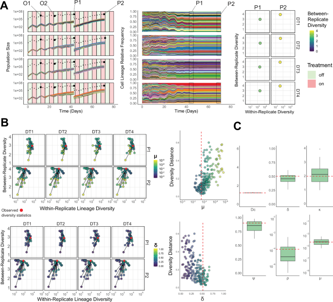
A Simulated population size (Left) and cell lineage (Middle) changes across 4 experimental drug-treatment replicates (DT1-4) and their lineage diversity statistics (Right). Total cell population size trajectories (dashed lines) and the top 20 lineage population sizes (coloured lines)/relative frequencies (shaded areas) across four experimental drug-treatment replicates (DT1-4, rows). Lineage colours are consistent between replicates. Four total cell size observations per replicate (two intermediate population size timepoints (O1 & O2) and two passage size timepoints (P1 & P2)) are highlighted. B A subset of the simulated lineage diversity statistics for each sub-population’s two timepoints (P1-2, rows) used for the parameter inference step, highlighted by one of the model parameters (Top: sensitive to resistant phenotype transition probability per cell division – μ) and the fitness penalty of resistance (Bottom: controlled by δ) compared to the true diversity statistics for the given simulation (red points). Adjacent panels show the normalised lineage diversity distance as a function of the two parameters, with the true parameter value highlighted (red dashed line). C Posterior distributions (n = 50, 4 experimental replicates) of the inferred parameter values using the combined cell population size and cell lineage statistics (true parameter values – red dashed lines). Boxplots show the median, the first and third quartiles, and whiskers 1.5x the interquartile range. Source data including the full list of parameters used for the simulation are provided as a Source Data file.
To assess the accuracy of our framework, we evaluated our ability to recover parameters from synthetic data where the true parameter values (ground truth) were known. For a specific set of parameters, we collected data on total population size changes and lineage distributions at predefined treatment times across four replicate sub-populations (Fig. 3).
When inferring parameter values without incorporating lineage distributions in the second step of our fitting procedure, we found that, while these observations could exclude many parameter combinations, a broad range of possibilities remained that the model could not distinguish (Supplementary Fig. 1B). Whilst population trajectories alone allowed us to recover the effective strength of treatment (Dc), the parameters governing the distribution of the resistant phenotype within and between cell lineages over time (such as μ and ρ) were poorly identified. Specifically, when resistance was rare in the cell population, the initial drop in population size at the early observation timepoint (O1) was mainly driven by the selection pressure on sensitive cells (as determined by Dc). However, the subsequent population rebound during treatment, driven by the emergence of predominantly resistant cells, could be explained by different combinations of pre-existing resistance (ρ) and phenotypic transition probabilities from sensitive to resistant (μ).
When performing inference using both sources of information, the lineage relationships at each timepoint – as described by the diversity statistics – increased the power to identify evolutionary parameters markedly (Supplementary Fig. 1D). For example, the addition of lineage information could distinguish between parameter combinations that led to similar overall proportions of resistance and sensitivity, but markedly different rates of phenotype switching (different μ values) and high fitness costs associated with resistance (different δ values) which cause selective lineage expansion and contraction (Fig. 3B, C). Repeating this model inference framework on parameter sets for each of our resistance models showed the approach could recover values from a range of evolutionary scenarios (Supplementary Fig. 2).
There were scenarios that led to treatment having a minimal impact on the cell population size, limiting the modelling framework’s ability to recover the ground truth parameters. This was the case if resistance was extremely common (e.g., high values of ρ) or if the strength of selection exerted by the drug was weak (low values of Dc). Notably, whilst both behaviours lead to an unresponsive population, they do so due to subtly different reasons. If resistance is common, there can still be a small fraction of sensitive cells that are killed during treatment, whereas a weak drug effect would kill all cells with an equally low probability. Since our modelling framework relies on the population size changes and relationships between surviving lineages to identify likely parameter combinations, these scenarios hindered accurate parameter recovery (Supplementary Fig. 3). These scenarios are less relevant to studying the dynamics of resistance evolution, as they represent situations where the population is essentially drug-resistant at the outset.
In model B, we found the framework usually failed to accurately identify the reversion switching probability from resistant to sensitive (σ) (Supplementary Fig. 2B). Given this switching led to cells reverting to the sensitive phenotype within previously resistant cell lineages, they were often then lost in subsequent treatment rounds, obscuring the behaviour’s impact. Higher values of the reversion switching probability (σ) have a similar impact on population composition as a lower strength of the resistant phenotype (ψ): cells that either were or are resistant are killed independent of their lineage identity due to a rapid reversion to sensitivity (σ) or a weaker resistant phenotype (ψ). In more detail: phenotype switches back to a sensitive state (controlled by parameter σ) lead to an overall increased rate of cell death for the lineage where the switch has occurred, and a reduction in the size of the lineage. Because phenotype switches occur at a uniform rate across all cell lineages, a higher rate of reversion back to the sensitive state has an identical effect to increasing the direct death rate of the resistant cells (lower ψ). Incomplete resistance may occur due to very rapid phenotypic shifts, for example due to the stochastic partitioning of transcripts during cell division49.
The framework also struggled to recover the model behaviours if diversity was lost too rapidly. Our inference relies on distinguishing possible evolutionary scenarios by identifying shifts in diversity statistics between sampling steps. If the selection pressure exerted by treatment was too strong, only one/a few barcodes remained in each replicate by the first sampling step and the statistical power to distinguish scenarios was lost.
We explored whether these difficulties could be addressed with newer ‘evolving barcodes’ that continuously generate novel barcode tags within cell lineages, enabling higher resolution reconstruction of cell phylogenies50. To explore the power of evolving barcodes in a simple setting we performed an additional re-barcoding step at the first passage (P1) to reintroduce measurable diversity into the system. We found that this information didn’t help solve the unidentifiability of the strength of resistance and reversion transition probability in Model B (σ vs ψ). However, in our Model C, it could help identify clonal sweeps due to ‘escape transitions’ that occurred following a complete loss of diversity prior to P1 (Supplementary Fig. 4).
The difficulties in recovering the reversion phenotypic transition probability (σ) were absent for the sensitive to resistant transition (μ) where the probability strongly dictates the number and identity of surviving lineages. Given this unidentifiability of Model B (‘bidirectional transitions’), we chose to focus on the differences between models A and C – unidirectional switching & escape transitions.
As well as identifying parameters within each of our models, we wanted to know when the framework could distinguish between them. We therefore simulated two sets of ‘ground truth’ scenarios using each of our models A and C (28; 14 per model) and compared their ability to recover the true evolutionary scenario. Due to the differing complexity of our models (as captured by the differing number of parameters), we used the Deviance Information Criterion (DIC), a measure of model fit that penalises for model complexity51.
We found there were cases where the differences left in the lineage distributions enabled the identification of the correct evolutionary model (as illustrated by a lower DIC score) (Supplementary Fig. 5): the data generated by the simpler model A (‘unidirectional’) were correctly identified for all of the scenarios investigated, whilst in over half of the cases where the true model was model C (‘escape transitions’) the model A (‘unidirectional switching’) was preferred; the evidence in favour of our more complex model (model C) had to be strong to confidently reject our simpler model (model A). Rejection of model A occurred when the transition to the ‘escape’ phenotype in model C led to stochastic crashes in diversity across replicates that could not otherwise be explained by the total cell population size changes (Supplementary Fig. 5B). These behaviours were observed when a moderate level of resistance (higher values of μ or ρ) with an associated fitness penalty (via δ) survived the initial rounds of treatment, and the probability of experiencing an escape transition (α) was relatively low.
In summary, for the scenarios explored here, we found that by combining commonly measured features of cell populations during long-term evolution experiments—cell population size changes and cell lineage distributions (summarised via diversity statistics)—we could recover parameters that govern the response of the population to treatment and the evolution of resistance phenotypes. Furthermore, we show that in certain scenarios there are statistical signatures left by our more complex model that allow us to distinguish it from a simpler model characterised by two phenotypes and unidirectional switching.
Experimental evolution of drug resistance in colorectal cancer
We applied our modelling framework to investigate the dynamics of resistance evolution in two common colorectal cancer cell line models: SW620 (a line exhibiting chromosomal instability (CIN)) and HCT116 (a mismatch repair deficient (MMRd) line).
To enable the tracking of cell lineage information, we labelled each cell line with a stable genetic barcode system (ClonTracer—Bhang et al.52). We refer to the barcoded cell lines as SW6bc (SW620) and HCTbc (HCT116). After growing cells for a short expansion step (~6 population doublings in HCTbc and 5 population doublings in SW6bc) to ensure most barcodes were represented multiple times, we split each cell-line’s barcoded parental population (POT) into control (CO1-4) and drug treatment (DT1-4) replicates and subjected each subpopulation to periodic treatments of vehicle control (DMSO) or IC50 concentrations of 5-fluoruracil (5-Fu) (a constituent part of standard-of-care colorectal cancer chemotherapy treatments such as FOLFOX) (Figs. 4A, 5A). We isolated and sequenced barcoded single cell colonies to ensure the majority of cells contained a single barcode (Supplementary Fig. 6). We combined cell counts and imaging to derive total cell population size estimates at four time points (O1,O2,P1,P2) per treatment replicate (DT1-4) within the first two passages and extracted and sequenced the heritable genetic barcodes to measure the cell lineage distributions at each passage (Supplementary Data 2 & Supplementary Data 3). We also used the distribution of lineages from the expanded, untreated cells (POT) to estimate the parental populations’ average birth and death rates for each cell line and used these estimates to parameterise the full resistance models (see Supplementary Note 1). We then fit our models of resistance evolution to the total cell population size estimates and lineage distribution data. Because we observed sustained lag times between the commencement of treatment and the first passage (P1) in both cell lines (SW6bc: +37 days; HCTbc: +67 days – Figs. 4B, 5B) we were confident that resistance was not already the dominant phenotype and that the selective pressure exerted by treatment was substantial.
Fig. 4: Quantification of the evolutionary dynamics during treatment in a barcoded colorectal cancer cell line (SW6bc).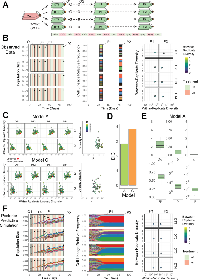
A A simplified schematic of the experimental design used in a long-term evolutionary resistance assay. Barcoded SW620 cells (SW6bc) were barcoded and expanded (POT) before being sampled into four replicate drug-treatment sub-populations (DT1-4) that were exposed to periodic chemotherapy treatment (5-fluoruracil: 5-Fu) and passaged at two timepoints (P1 & P2). B Population size counts at four timepoints per-replicate (DT1-4), including two intermediate population size estimates (O1 & O2) and two Passage timepoints (P1 & P2) (left panel); top 20 sequenced barcode lineage relative frequencies at the two passage timepoints, where area colour denotes lineage identity (middle panel); lineage diversity statistics of the sequenced barcode distributions at the two passage timepoints (P1 and P2) for each replicate composed of within replicate lineage diversity and between-replicate diversity dissimilarity. C Posterior predictive simulations for Model A (unidirectional transitions–top) and Model C (escape transitions – bottom) of the within and between-replicate diversity statistics (LHS) and the normalised diversity distance from the observed statistics (red points) to the simulated values (highlighted by the transition parameter μ). D The Deviance Information Criterion (DIC), a measure of model fit, for Model A & Model C (lower values indicate higher model support) calculated using the posterior predictive distributions. E The posterior distributions (n = 50, 4 experimental replicates) for parameters in Model A (the model with the highest support). Boxplots show the median, the first and third quartiles, and whiskers 1.5x the interquartile range. Parameters: ρ—pre-existing fraction of resistance, μ—sensitive to resistant transition probability per cell division, ψ— strength of the resistant phenotype, Dc—maximum strength of the drug, κ—accumulation/decay rate of the drug. F A posterior predictive simulation using Model A. Source data are provided as a Source Data file.
Fig. 5: Quantification of the evolutionary dynamics during treatment in a barcoded colorectal cancer cell line (HCTbc).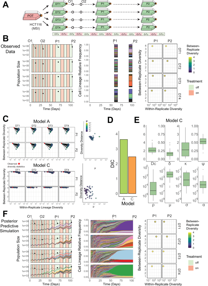
A A simplified schematic of the experimental design used in a long-term evolutionary resistance assay. Barcoded HCT116 cells (HCTbc) were barcoded and expanded (POT) before being sampled into four replicate drug-treatment sub-populations (DT1-4) that were exposed to periodic chemotherapy treatment (5-fluoruracil: 5-Fu) and passaged at two timepoints (P1 & P2). B Population size counts at four timepoints per-replicate (DT1-4), including two intermediate population size estimates (O1 & O2) and two Passage timepoints (P1 & P2) (left panel); top 20 sequenced barcode lineage relative frequencies at the two passage timepoints, where area colour denotes lineage identity (middle panel); lineage diversity statistics of the sequenced barcode distributions at the two passage timepoints (P1 and P2) for each replicate composed of within replicate lineage diversity and between-replicate diversity dissimilarity. C Posterior predictive simulations for Model A (unidirectional transitions–top) and Model C (escape transitions – bottom) of the within and between-replicate diversity statistics (LHS) and the normalised diversity distance from the observed statistics (red points) to the simulated values (highlighted by the transition parameter μ). D The Deviance Information Criterion (DIC), a measure of model fit, for Model A & Model C (lower values indicate higher model support) calculated using the posterior predictive distributions. E The posterior distributions (n = 50, 4 experimental replicates) for parameters in Model C (the model with the highest support). Boxplots show the median, the first and third quartiles, and whiskers 1.5x the interquartile range. Parameters: ρ – pre-existing fraction of resistance, μ—sensitive to resistant transition probability per cell division, σ— resistant to sensitive transition probability per cell division, α—resistant to escape transition probability per cell division, ψ—strength of the resistant phenotype, Dc—maximum strength of the drug, κ—accumulation/decay rate of the drug. F A posterior predictive simulation using Model C. Source data are provided as a Source Data File.
In the barcoded cell line SW6bc, fitting our model A (‘unidirectional switching’) predicted that resistance was rare when the experiment began (ρ = 1.1×10⁻⁴ ± 2.3×10⁻⁴, mean ± s.d.) and that the phenotypic transition probability from sensitive to resistant was low (μ = 7.6 × 10⁻⁷ ± 1.5 × 10⁻⁶, mean ± s.d.). Resistant cells also experienced a significant probability of drug-induced death during treatment (ψ = 0.63 ± 0.01, mean ± s.d.) and the fitness penalty of resistant cells in the absence of treatment was moderately low (δ = 0.11 ± 0.08, mean ± s.d.) (Fig. 4E, and Supplementary Data 4). These dynamics led to resistant lineages that were not dominant in the population until the end of the 2nd passage, as illustrated by the drop in within-replicate diversity between P1 and P2 (Fig. 4C, Top). The ‘unidirectional’ model was preferred over the more complicated ‘escape transition’ model, as supported by a lower DIC score (Fig. 4D). The low frequency of resistance and its stability through cell divisions predicted by the model explain the high similarity of the lineage distributions (low between-replicate diversity values, Fig. 4B, F, right hand column): the correlation between lineage identity at the time of barcoding (t0) and the resistant phenotype remains largely unbroken through multiple rounds of treatment and population bottlenecks. The dynamics predicted by the modelling framework were consistent with a stable, pre-existing resistance mechanism that emerges gradually from a predominantly sensitive population in SW6bc.
In our second barcoded cell line, HCTbc, a few different unique lineages grew to dominate each replicate flask following treatment for two passages (Fig. 5B). To recover the population size changes and unique barcodes ‘winning’ across each replicate sub-population, we had to invoke our more complex model C, ‘escape transitions’ (Fig. 5C, D).
The model supported resistant cells incurring a fitness penalty (δ = 0.18 ± 0.08, mean ± s.d.) and there was a high probability of a transition from the sensitive to resistant phenotype per cell division (μ = 7.6 × 10⁻² ± 0.11, mean ± s.d.). The probability with which cells escaped the fitness penalty was lower (α = 2.5 × 10⁻⁴ ± 6.8 × 10⁻⁴, mean ± s.d.) (Fig. 5E, Supplementary Data 5). These dynamics led to sensitive cells having a moderate but equipotent capacity to switch to a slower growing resistant phenotype to survive initial rounds of treatment, followed by rarer ‘jackpot’ events where lineages grew to dominate the population after escaping the fitness penalty (α). The lower probability of these jackpot events occurring within slower growing resistant cells also contributed to stochastic variation in diversity statistics between replicates (Fig. 5C, Bottom Panel), as observed in our sequenced barcode distributions.
This ‘two-stage’ evolutionary process predicted to be responsible for resistance in our barcoded HCTbc cell line is reminiscent of ‘persister’ dynamics observed elsewhere, whereby a population of cells with slower division rates initially survive treatment and provide a reservoir of cells within which additional adaptive changes can accrue6,53,54,55.
In HCTbc, the model predicted the rate at which cells experience elevated death rates due to the change in effective drug concentration (κ) to be quicker compared to SW6bc. This difference meant the relative fitness benefit experienced by the resistant (vs sensitive) phenotype immediately following treatment was greater in HCTbc, consistent with the greater relative increases in the IC50 values for the HCTbc drug-treatment replicates (Supplementary Fig. 7).
In summary, data from the SW6bc cell line were best explained by model A (unidirectional transitions), where resistance was rare and the transition rate from sensitive to resistant cells was low, consistent with a stable, pre-existing molecular driver of resistance. In contrast, data from the HCTbc cell line were better predicted by model C (escape transitions), where faster-growing, treatment-resistant cells emerged from a more common population of slower-growing, treatment-refractory cells.
Functional characterisation of resistant cells verifies modelling inferences
We performed detailed molecular and functional characterisation of cells from our long-term resistance evolution experiment conditions. Whilst our framework does not infer the molecular mechanisms of resistance directly, it does make predictions for how the phenotypes (here, resistance to our chemotherapy 5-fluorouracil) should be distributed amongst a cell population.
To test the predictions generated from our modelling framework at the transcriptional level, we performed single-cell RNA sequencing (scRNA-seq) of the expanded parental population (POT), two fourth passage control (CO), two fourth passage drug-treatment (DT) replicates and two ‘drug-stop’ (DS) replicates (Fig. 6A). The DS replicates had only been subject to a single cycle of treatment and recovery before being harvested and hence primarily exhibited the phenotype of treatment-exposed parental cells. We could therefore compare DS and DT conditions to the parental (POT) samples simultaneously to isolate gene expression changes that were either: an ‘acute treatment response’ following recent exposure to the drug (changes shared between DS and DT comparisons); a ‘sensitive treatment response’ in genes that were only found differentially expressed when the ancestral population was exposed to treatment (differentially expressed in DS but not DT comparisons); and a ‘resistance treatment response’ for genes differentially expressed in the evolved resistant lines but not the sensitive parental cells (differentially expressed in DT but not DS comparisons). Given these comparisons, gene expression changes associated with resistance can fall into two categories: either those that are found solely differentially expressed in the drug-treatment replicates (‘resistance treatment response’) or those whose differing expression in response to acute treatment exposure in the sensitive population has been lost during the evolution of resistance in the drug-treatment replicates (‘sensitive treatment response’).
Fig. 6: Functional characterisation of resistance in SW6bc.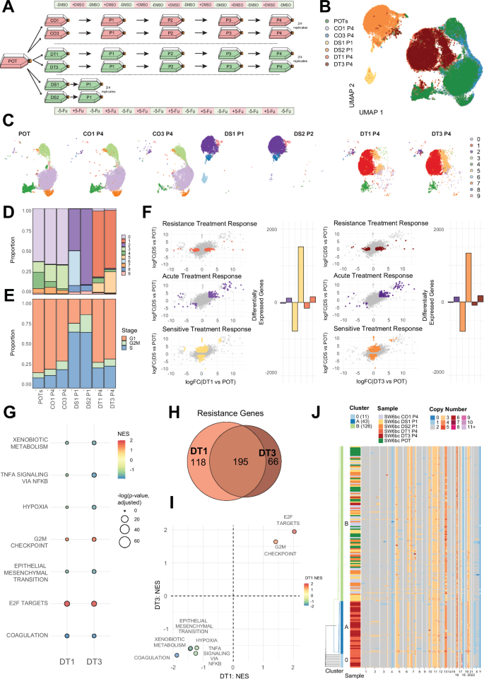
A Schematic of sample design and naming schemes from the long-term resistance evolution experiment using barcoded SW620 colorectal cancer cells. Periods of on/off treatment (5-Fu and DMSO) are for illustrative purposes and are not to scale. B UMAP dimensionality reduction of the scRNA-seq data from chosen sample replicates. C Cluster assignment of UMAP results on a sample-by-sample basis highlighted by cluster identity. D Cluster assignment proportions by cell sample. E Cell cycle stage proportions by cell sample. F Genes associated with replicate-specific differential expression (DE) identified via specific comparisons (coloured points per panel): Resistance Treatment Response – DE in DT but not DS; Acute Treatment Response – DE in DT and DS; Sensitive Treatment Response – DE in DS but not DT. Comparisons are performed for each drug treatment replicate (DT1 & DT3), and the number of significantly DE genes in each group are also shown per comparison. Significantly differentially expressed genes were identified using a quasi-likelihood F-test (QLF test) in edgeR. G Gene set enrichment analysis (GSEA) for each drug-treatment replicate (DT1 and DT3) for genes identified as ‘Resistance’ genes in each replicate. Only gene sets that were found to be significant (adjusted p-value p-values were computed using the multilevel adaptive algorithm implemented in fgseaMultilevel. H The number of shared/unique Resistance genes between each drug-treatment replicate. I ‘Resistance’ genes GSEA NES comparison between DT1 and DT3. J A subset of single-cell copy number profiles from SW6bc experimental replicates. Each row is a single cell and chromosome bin colour denotes copy number. Rows are highlighted by sample identity and cluster assignment. Source data is provided as a Source Data file.
In our barcoded SW6bc CRC cell line (Supplementary Data 6), our modelling framework predicted the existence of a pre-existing, stable molecular driver of resistance. The parental and control replicates exhibited highly similar expression profiles, supporting the experimental passaging and vehicle control treatment having a negligible effect on gene expression (Fig. 6B, C). The drug-treatment replicates also exhibited remarkably similar expression profiles with each other, despite several months of chemotherapy in isolated experimental replicates (Fig. 6C). Of the differentially expressed genes associated with resistance (Fig. 6F – ‘resistance treatment response’ signature), the majority were shared between the two sequenced replicates (Fig. 6H). Furthermore, the shared nature of gene expression was also present when comparing gene signature hallmarks, with high concordance in the normalised enrichment scores (NES) (Fig. 6G, I). Most gene expression differences across all comparisons in SW6bc were those unique to the DS replicates (Fig. 6F – ‘sensitive treatment response’ signature). Given DT and DS replicates have both been recently exposed to the chemotherapy 5-Fu, these findings suggest that evolution of resistance in SW6bc leads to cells that more closely resemble their untreated ancestors despite ongoing treatment. Overall, the scRNA-seq results described here are consistent with selection for a shared resistant phenotype across replicates, as predicted by our modelling results.
Given the putative chromosomal instability in this cell-line, we also looked for evidence supporting the selection of a rare pre-existing sub-population with a unique pattern of copy number alterations (CNAs) by measuring CNAs in individual cells. We performed single-cell shallow whole-genome sequencing via ‘Direct Library Preparation’ (DLP) on different cells from the same experimental conditions that were characterised via scRNA-seq56. The copy-number profiles supported ongoing chromosomal instability in SW6bc, with small sub-clonal changes found across all samples (Fig. 6J). Consensus copy number profiles derived using all cells within a sample identified additional changes shared by only the drug-treatment replicates (Supplementary Fig. 8), consistent with the repeated selection of a shared ancestral lineage (as seen in the lineage tracing and transcriptomic data). Clustering based on the single-cell copy number profiles grouped most cells from each drug-treatment replicate (DT1 & DT3) together, also consistent with the expansion of a shared ancestral sub-clone (Fig. 6J).
In our second barcoded CRC cell line, HCTbc (Supplementary Data 7), we performed scRNA-seq on replicates with the same sample design as our previous cell-line (Fig. 7A). Whilst the high concordance between POT and CO replicates again supported a minimal impact of sampling and vehicle control treatment, the two replicates’ drug-treatment cells exhibited markedly distinct expression profiles (as represented via dimensionality reduction; UMAP – Fig. 7B, C). Also, in contrast to SW6bc, the DS replicates were enriched for the G1 cell cycle stage, consistent with elevated cell-cycle arrest in parental cells following a single round of treatment.
Fig. 7: Functional characterisation of resistance in HCTbc.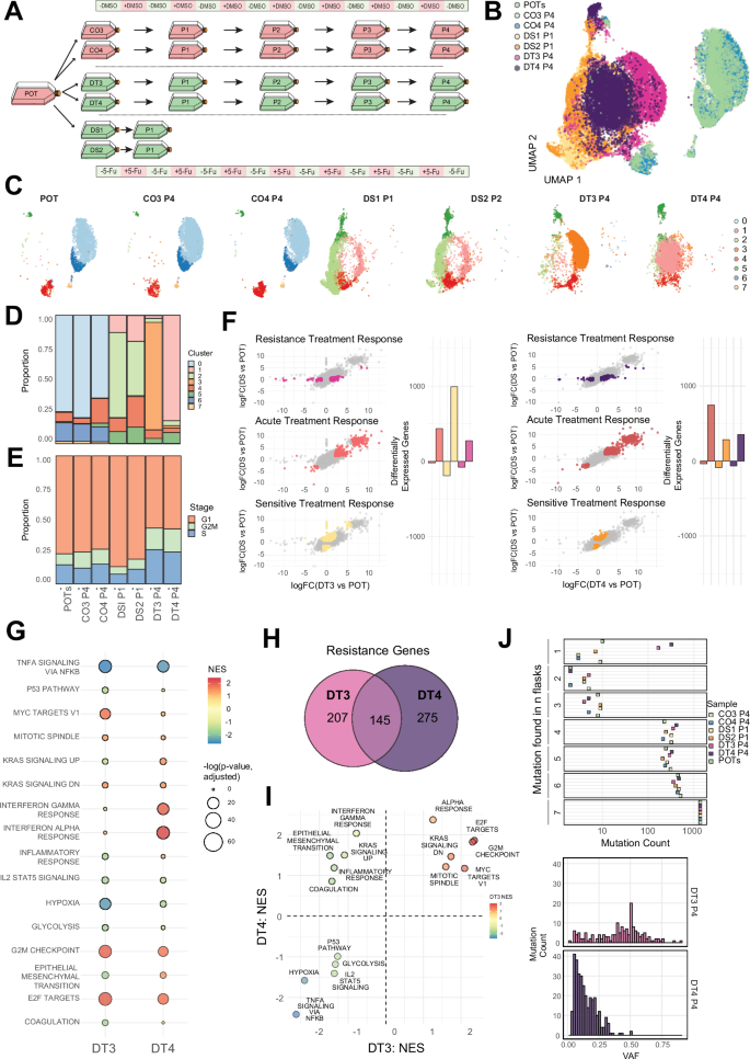
A Schematic of sample design and naming schemes from the long-term resistance evolution experiment using barcoded HCT116 colorectal cancer cells. Periods of on/off treatment (5-Fu and DMSO) are for illustrative purposes and are not to scale. B UMAP dimensionality reduction of the scRNA-seq data from chosen sample replicates. C Cluster assignment of UMAP results on a sample-by-sample basis highlighted by cluster identity. D Cluster assignment proportions by cell sample. E Cell cycle stage proportions by cell sample. F Genes associated with replicate-specific differential expression (DE) identified via specific comparisons (coloured points per panel): Resistance Treatment Response – DE in DT but not DS; Acute Treatment Response – DE in DT and DS; Sensitive Treatment Response – DE in DS but not DT. Comparisons are performed for each drug treatment replicate (DT3 & DT4) and the number of significantly DE genes in each group are also shown per comparison. Significantly differentially expressed genes were identified using a quasi-likelihood F-test (QLF test) in edgeR. G Gene set enrichment analysis (GSEA) for each drug-treatment replicate (DT3 and DT4) for genes identified as ‘Resistance’ genes in each replicate. Only gene sets that were found to be significant (adjusted p-value p-values were computed using the multilevel adaptive algorithm implemented in fgseaMultilevel. H The number of shared/unique resistance genes between each drug-treatment replicate. I ‘Resistance’ genes GSEA NES comparison between DT3 and DT4 (J) Mutations found in scRNA-seq data grouped by the number of replicate flasks any mutation was found in and VAF distributions of mutations found in scRNA-seq data unique to the two drug-treatment replicates. Source data are provided as a Source Data file.
In one of the two drug-treatment replicates characterised (DT3), the majority of differentially expressed genes across our joint comparisons were those that were only found in the parental cells’ response to treatment (DS – ‘acute treatment response’, Fig. 7F). However, unlike SW6bc, the other replicate (DT4) shared a higher proportion of differentially expressed genes with the parental population’s response to treatment (POT vs DS and POT vs DT – ‘acute treatment response’, Fig. 7F). These suggest that one of the two replicates (DT3) now more closely resembles the untreated ancestral phenotype (POT) despite ongoing treatment. Alongside most resistance associated genes being unique to each drug-treatment replicate (Fig. 7H), these results supported the emergence of unique resistant phenotypes in HCTbc. Interestingly, in contrast to SW6bc, this non-repeatability was observable when comparing hallmark gene sets: whilst some pathways showed concordance in the magnitude and direction of enrichment, some pathways showed different directions between the two replicates, including EMT genes and genes associated with elevated KRAS signalling (both showed elevated enrichment in DT4 but depletion in DT3 – Fig. 7I).
As HCTbc was characterised by microsatellite instability, we investigated the clonal dynamics associated with resistance evolution by comparing the mutational landscape of the cells (called from scRNA-seq data). We compared the number of mutations found in n of the total sequenced replicate flasks (Fig. 7J). Many mutations were found that were unique to each drug-treatment replicate (Fig. 7J– Found in 1). Comparison of the VAF distributions supported more complete dominance of the ‘jackpot’ lineage (predicted by the modelling) in the DT3 replicate, where a large number of mutations had reached clonality (VAF ~ 0.5), whereas in DT4 the stochastic nature of the successful lineage emergence had either led to clonal interference mitigating clonal dominance, or incomplete dominance of the faster proliferating resistant lineage in the population. This latter hypothesis was supported by a ‘fitness assay’: single cell isolated clones derived from DT4 were significantly slower growing than those from DT3 (Supplementary Fig. 9), and the transcriptional results which also supported DT4 more closely resembling the phenotype of the parental cells recently exposed to treatment (the DS condition).
Our modelling framework predicted evolution during treatment in HCTbc occurred via a two-step process: treatment refractory cells that exhibited a fitness penalty (realised as slower net growth rates) initially survived treatment (the ‘resistant’ phenotype), and cells that escape this fitness penalty but remained resistant emerged stochastically from this population as treatment continued (the ‘escape’ phenotype). We reasoned that our original scRNA-seq sampling design alone was limited in its ability to distinguish these dynamics from other evolutionary scenarios. Specifically, because the transition to ‘escaped’ was predicted to have occurred between seeding and the first passage, waiting for the cells to fill the flask means observations were limited to cells that had emerged following the second event.
Motivated by this, we performed an additional drug-treatment experiment where we exposed parental barcoded cells (HCTbc POT) to periodic chemotherapy using the treatment regime adopted during our original experiment. We waited until colonies of cells appeared that could readily proliferate despite ongoing treatment, and we observed that when this occurred the dividing cells were smaller than the majority of those that had initially survived treatment (Supplementary Fig. 10A). We therefore predicted we could use size as a proxy for cells occurring pre- and post- the ‘escape’ event and isolated single small or large cells before performing scRNA-seq. We also sequenced (scRNA-seq) single cells from the original HCTbc experimental conditions (Fig. 6A) to validate these new comparisons.
To identify differentially expressed genes relative to the parental (POT) cells but either shared with or independent of the parental population’s response to treatment (DS), we performed analogous comparisons to those discussed previously to identify a signature of: ‘large cell treatment response’ (changes associated with large cells but not DS replicates); ‘small cell treatment response’ (changes associated with small cells but not DS replicates); ‘acute treatment response’ (changes associated with either large or small cells and DS replicates); and ‘sensitive treatment response’ (changes associated with the DS replicates but not either large or small cells). Whilst the large cells exhibited the highest number of differentially expressed genes in response to treatment vs the DS replicates, performing these comparisons with the small cells revealed a high number of genes in the ‘sensitive treatment response’ group (Supplementary Fig. 10B). Finding the majority of differentially expressed genes unique to the DS replicates was consistent with the emergence of a readily proliferating small cell phenotype that more closely resembles the ancestral (POT) cells. Correlations between average cell expression profiles also support a small cell phenotype that more closely resembles the parental cells, whereas the large cells appear transcriptionally distinct (Supplementary Fig. 10C). Interestingly, gene set enrichment analysis on genes that were differentially expressed in the large cells (relative to the POT replicates) showed down regulation of pathways that were elevated in the HCTbc drug-treatment replicates (Supplementary Fig. 10D). In contrast, these pathways were up-regulated in the small cell phenotype (Supplementary Fig. 10E), consistent with the drug-treatment replicates. These findings supported two distinct phenotypes existing following treatment in HCTbc, as predicted by our model. Whilst we cannot be certain that the presence of large and small cell phenotypes are indicative of a process whereby the latter emerges from the former, the existence of distinct colonies who have gene expression changes that more closely resemble resistant cells suggest rare, stochastic changes render cells able to proliferate despite the presence of treatment.
In summary, our functional characterisation of cells derived from the same experiment used to infer evolutionary dynamics from population size data and lineage distributions supported the predictions made by our modelling framework. In SW6bc (a CIN barcoded CRC cell line) a simple model of a stable, pre-existing molecular driver of resistance was most likely. In contrast, in HCTbc (a MSI barcoded CRC cell line), a more complicated two-step model was required to explain the data.