Physical encoder
Most ultraintense lasers approximate an ideal top-hat intensity profile in the near field, which when focused with a perfect lens, form an Airy ring in the far field, with 95% of the energy contained within the first four Airy rings and less than 1% of the total energy in the fifth (Supplementary Section 1). According to the Nyquist criterion, resolving this spatial range in the far field requires two measurement points per ring, resulting in an 8 × 8 sampling grid in the near field. High-frequency features that would be captured with a larger sampling rate in the near field will end up outside this region of interest in the far field.
This sampling rate is far smaller than is typically aimed for in ultraintense laser characterization, and provides an opportunity to trade-off the spatial resolution of the sensor to capture the information of different dimensions. Here an optical system is proposed (Fig. 1a) to encode the phase, spectral and polarization information into the intensity before it is captured by the sensor. The final design reaches more than twice the resolution required to capture the first four Airy rings, and for an f/50 optic at a central wavelength of λ0 = 800 nm corresponds to a measurement area of about 1 mm2, which is almost 700 times the ideal waist size \(\uppi {w}_{0}^{2}\). Furthermore, considering a spectral range of Δλ = 100 nm, one is able to resolve tmax = 100 fs in the far field with ten samples; RAVEN achieves a resolution of at least double this value.
Fig. 1: The RAVEN technique to perform single-shot measurements of vector fields.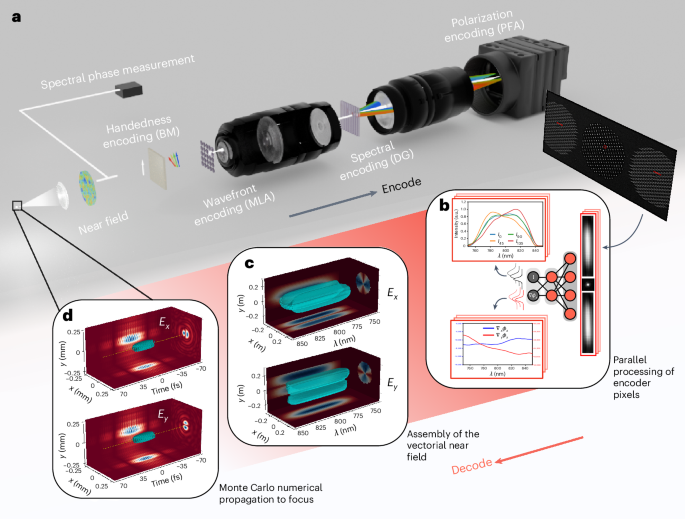
a, Optical setup task encodes the four-dimensional vector field onto a two-dimensional intensity measurement (not to scale). The collimated beam is split, with one part used to measure the spectral phase and the rest passing through a birefringent medium (BM), creating a relative spectral chirp between the polarizations. Next, a microlens array (MLA) encodes the wavefront. The resulting pattern is imaged by a 4f system with a diffraction grating (DG) placed near the Fourier plane, providing the spectral encoding, and a polarization filter array (PFA) is used on the sensor. b, Extraction and processing of the encoding pixels. At each point in space, the spectral and polarization information is recovered, with uncertainty estimates. c, Aggregation of the information from the encoder pixels into the vectorial near field. d, Propagation to focus.
The design begins with the Shack–Hartmann sensor29. A common way to simultaneously capture the monochromatic intensity and phase of a laser pulse is by a microlens array, which locally samples the wavefront in many locations and encodes the average phase gradient over each sub-aperture into the resulting shifts of the focal spots. This averaging is crucial, as it both reduces aliasing from higher-frequency components and leads to a better signal-to-noise ratio compared with other phase-encoding methods, for example, the pinhole-based Hartmann sensor. To extend this to a hyperspectral setting, the plane of the focii is imaged using a 4f system, with a diffraction grating placed close to the Fourier plane. The resulting diffraction pattern at the sensor is composed of the fundamental order, as well as the ±1 orders, resulting in a kind of sparse tomography. Crucially, the ±1 orders obtain chromatic dispersion, thereby encoding the spectral information in streaks at the detector. Analogous to tomographic reconstruction, we can see these as projections of our hyperspectral intensity. One notes that it is necessary to have both ±1 orders, as with just one, there exists an ambiguity between the spectral intensity and phase.
To capture the full information of the polarization state and, thus, the four Stokes parameters, one must acquire the magnitudes of the field in two orthogonal directions, namely, ∥Ex∥ and ∥Ey∥, and the relative phase delay between them, δ. Here a camera with a polarizing filter array is used, which gives the spatial intensity for filters arranged in directions ∈ (0°, 45°, 90°, 135°). The field magnitudes are found as the square root of the 0° and 90° components. The magnitude of polarization delay is found by
$$\pm \delta =\arccos \left(\frac{{I}_{135}-{I}_{45}}{2\sqrt{{I}_{0}{I}_{90}}}\right),$$
where I is the intensity, but crucially, its sign is still unknown30. Resultingly, the fourth Stokes parameter is only known to a plus–minus ambiguity, corresponding to an insensitivity to the handedness of the polarization state.
Here this is resolved by the prior knowledge of the signal’s sparsity, and the use of a precharacterized birefringent medium placed before the microlens. This element adds a further delay between the polarizations, δB, so that the final delay at the sensor is δM = δ + δB. From the assumption of the initial field’s smoothness, it follows that its initial spectral variation of the polarization delay, that is, \(\left\Vert \frac{\partial \delta }{\partial \lambda }\right\Vert\), is small. One chooses a birefringent medium that causes a large temporal chirp between the polarizations, such that \(\left\Vert \frac{\partial {\delta }_{{\rm{B}}}}{\partial \lambda }\right\Vert \gg \left\Vert \frac{\partial \delta }{\partial \lambda }\right\Vert\). When a measurement is taken, two ambiguous solutions are found, ±δM. Here one selects the solution whose spectral gradient is in the same direction as that of the birefringent medium. Subsequently, subtracting the precalibrated δB yields the initial field’s polarization delay δ. An example of a suitable birefringent medium is a multiorder half-wave plate, but with prior knowledge of the pulse’s expected polarization state, one can choose a medium to maximize the intensity in all four polarization channels to improve the signal-to-noise ratio.
Software decoder
Due to the unique encoding achieved by the optical setup, the system is theoretically bijective. However, real-world measurements invariably contain noise, which complicates the reconstruction process. Although convex optimization techniques could be used, they are typically slower and less adept at handling noise and uncertainty estimation. Thus, to achieve a real-time diagnostic capability that matches the repetition rate of ultraintense laser systems, neural networks are used. This approach not only provides rapid reconstruction (taking x, y, λ/t) are suppressed for brevity as they apply to every variable—conversely, where the indices are shown, they are the sole indices.
The reconstruction process begins by the extraction and subsequent analysis of the encoder pixels. These are formed of the microlens focii in the fundamental order (found using a peak finder), and the streaks in the ±1 orders, extracted using the precalibrated dispersion curve of the grating. The encoding pixels are then analysed in parallel by a fully connected deep neural network, which makes a prediction for the intensity in each polarization axis, I = [I0, I45, I90, I135], and the derivatives of the wavefront, \({\boldsymbol{\nabla }}{{\bf{\upphi }}}_{{\boldsymbol{x}}}=\left[\frac{\partial {\phi }_{x}}{\partial x},\frac{\partial {\phi }_{x}}{\partial y}\right]\), at each wavelength λ. By assuming a distribution of the uncertainty, one can train a network to estimate both values and their uncertainty, by minimizing the negative log-likelihood31,32. Here the standard Gaussian is used for the wavefront derivatives, and the folded Gaussian33 is used on the intensity to ensure that values below 0 are forbidden.
The vectorial near field is then formed by the synthesis of the encoding pixels. The phase derivatives for each wavelength are stitched together utilizing the zonal approach34, yielding \({{\phi }^{{\prime} }}_{x}\). To obtain the spatiotemporal phase, the spectral phase must also be added: \({\phi }_{x}={{\phi }^{{\prime} }}_{x}+\tilde{\phi }(\lambda )\). The polarization delay δ is extracted from the intensity predictions, as described above, so that ϕy is then found as ϕy = ϕx – δ, without the need of a separate spectral phase measurement in the other polarization direction. The result of this analysis is the complete near field with uncertainty estimates.
It is the field at focus which is of the most physical importance. Thus, the measured near field, along with its uncertainty estimates, is numerically propagated to the focus. To propagate the uncertainty estimates, Monte Carlo sampling is used. For a number of iterations, the near field is sampled from its distribution and propagated to the far field, which is stored. Finally, the uncertainty of the field at focus is approximated as a Gaussian, by the calculation of the mean and standard deviation of the samples for each point in the spatiotemporal volume. The same process is applied to the desired derivatives of the field at focus, such as calculating the peak intensity. The following results use a Fresnel propagator since the pulses under scrutiny are focused with a long focal length. However, the spatiotemporal foci under strong focusing and the resulting longitudinal fields can also be reproduced using a Rayleigh–Sommerfeld propagator.
MeasurementsSingle-shot measurement of ultraintense laser pulses
The RAVEN technique was used to perform the single-shot measurements of the spatiotemporal vector field of petawatt-class laser pulses. Measurements were performed at the ATLAS-3000 facility, which, during our beamtime, generated pulses with up to 35-J energy and a pulse duration of 29.6 fs. The RAVEN characterization results are displayed in Fig. 2. Although all the polarization information is measured, only the field along the ATLAS’ main polarization axis is shown.
Fig. 2: Single-shot measurement of the spatiotemporal field of a petawatt-class laser pulse.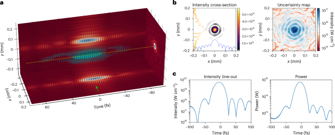
a, Electric field of an ATLAS-3000 pulse at focus. The visualization shows the isosurface of the field, where the carrier frequency has been reduced by factor of 2 for clarity. b, Temporal slice of the intensity at the centre of the beam (marked by the green arrow in a), along with its uncertainty estimate. Also included in the intensity slice are spatial line-outs through the centre of the cross-section, shown in the log scale. c, Intensity line-out through the centre of the beam, shown by the yellow line in a, and the power found by integrating the intensity over space. All the displayed error bars represent the predicted ±2σ confidence interval.
The resulting spatiospectral field at focus is shown in Fig. 2a, whereas a cut at t = 0 is shown in Fig. 2b. Note that the relative uncertainty at the peak intensity is two orders of magnitude lower than the signal level. Figure 2c shows the temporal intensity of the pulse, both at the focus position, (x = 0, y = 0), and integrated over space. The pulse duration of the former was found to be 29.8 ± 0.2 fs, in accordance with the previously quoted value. We calculated the spatiotemporal Strehl ratio of the laser (Methods)35, which is a reduction in the peak intensity due to the wavefront. The absolute ratio was 0.81 and the STC-isolated ratio (taken by removing the spectrally averaged wavefront from the pulse) was 0.93. These values are similar to those quoted at other petawatt facilities36.
After showing that RAVEN is able to resolve individual laser pulses, an experiment was performed to monitor, in real time, the STC content of the laser. Here the ATLAS-3000 system was operating at a 1-Hz repetition rate, whereas the pump energy was changed approximately every 20 min by changing the pump laser configuration. For each laser shot, RAVEN was used to acquire the pulse’s structure. We then calculate both STC content and STC-isolated spatiotemporal Strehl ratio, allowing the long-term dynamics of these changes to be studied. For these measurements, a reference was not taken, which means that the Strehl ratio includes the STCs induced by the optical system used to transport the pulse to RAVEN and is, thus, reduced compared with the true value. However, the dynamics can still be studied.
Figure 3 displays the evolution of the spatiotemporal Strehl ratio, along with the two STCs with the highest Pearson’s correlation coefficient with this ratio, namely, the pulse-front tilt in the horizontal direction (PFTx) and the pulse-front curvature (PFC). It is apparent that the hyperspectral Strehl ratio generally improves with the pump energy; intuitively, this is due to the fact that the compressor is aligned at one pump energy for which the pulse-front tilt is minimized with an inverted field autocorrelator37. Of all the STCs, it was found that PFTx was the most strongly correlated to the peak intensity (Pearson’s correlation coefficient ρ = 0.92).
Fig. 3: Evolution of the spatiotemporal Strehl ratio and STCs, with changes in the laser pump energy.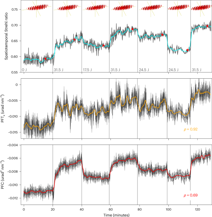
At each vertical grey line, the pump energy was changed, as denoted at the bottom of the spatiotemporal Strehl ratio subplot. Each red star denotes the temporal location in which the field is shown in the three-dimensional plot above. This measurement was not referenced, and thus, the spatiotemporal Strehl ratio includes contributions from STCs of the optical setup used to transport the pulse to the RAVEN setup.
PFC was also highly correlated, which displayed the property of stabilizing over relatively long time periods. This can be seen especially in the case when all the pump lasers were turned on, after they had all been off (T = 20 min). An explanatory candidate for this effect is the inhomogeneous heating of the gain medium as the pump energy was adjusted, and the subsequent change in thermal lensing38. This lensing is in itself chromatic and will, thus, result in different pulse-front curvatures. To our knowledge, these subtle dynamics have not been previously observed, even though they have a non-negligible influence on the focused intensity, characterized by the spatiotemporal Strehl ratio.
Vector field characterization of optical vortices
To demonstrate the full capabilities of the RAVEN technique, an experiment was conducted to measure a laser pulse that requires a vectorial treatment. The optical vortex is a type of vector field that has the intriguing property of possessing orbital angular momentum, manifested by a spiral wavefront, which leads to the formation of the characteristic ‘doughnut’ focus on propagation. These attributes make it of high interest in many experiments in the high-intensity regime39,40,41. Existing methods to characterize such fields have typically been developed for high-repetition-rate systems, requiring a scan with many laser shots42,43.
Here a quarter-wave plate was used to circularly polarize the incoming laser pulse, before it passed through a vortex retarder, imparting the pulse with orbital angular momentum (m = 2). Considering the pulse in terms of its polarization components Ex and Ey, each possessing a spiral wavefront, with a \(\pm \frac{\uppi }{2}\) phase shift between them, with the sign depending on the handedness of the circular polarization. RAVEN utilizes a spectrally dependent birefringent medium (in this case, a simple half-wave plate), and the prior assumption of spectral smoothness to determine the handedness. Due to beamtime restraints, this experiment was performed on an ultrafast oscillator, but there is no reason why this would not work at an ultraintense facility. The results shown in Fig. 4 demonstrate the spectral dependence of the resultant vector field, as expected, due to the chromatic properties of the quarter-wave plate and vortex retarder used to generate it.
Fig. 4: Single-shot measurement of the spatiotemporal vector field of an optical vortex.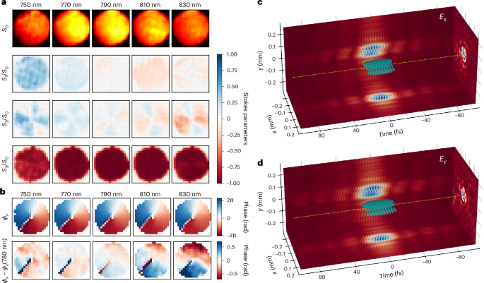
a, Spatiospectral Stokes parameters of the vectorial near field. b, Spiral wavefront of the optical vortex. The relative change from the design wavelength of the vortex retarder (780 nm) is also shown, displaying the chromatic properties of this object. c,d, Field at focus, for both Ex and Ey. The carrier frequency has been reduced by a factor of 2 for clarity, and the spatial units have been scaled to the ATLAS-3000 system (27-cm diameter in the near field).
In the case of a perfect left-handed circularly polarized beam44, the final three normalized Stokes’ parameters have the values
$$\frac{1}{{S}_{0}}\left[\begin{array}{c}{S}_{1}\\ {S}_{2}\\ {S}_{3}\end{array}\right]=\left[\begin{array}{c}0\\ 0\\ -1\end{array}\right].$$
Clear deviations from these values are seen as one moves away from the central wavelength of the laser because the quarter-wave plate is designed to create circularly polarized light at the design wavelength. Away from this, the polarization state will instead be elliptical. Similarly, one sees that deviations from the design wavelength of the vortex retarder leads to vortices being formed with non-integer orbital angular momentum.