We conducted a retrospective, ecological analysis of the count of incident cases of infection by SARS-CoV-2 within the Auvergne-Rhône-Alpes French region, to assess the association between infection rate and socio-economic indicators from census data. The study region accounted for 12% of the total metropolitan French population, with 8.1 million inhabitants in 2022. Our study was conducted for a time period between May 13th, 2020 and February 14th, 2021, covering most of the second wave in France. The study time frame was divided in four epidemics periods matching the dynamic of the second wave: a low incidence period up to July 26th 2020, the second wave growth phase up to October 25th, the peak and decrease period marked by local curfews followed by a national confinement up to December 13th and the stabilization phase up to February 14th 2021. No confinement or curfews were in effect aside from the third period, which starts at the epidemic peak of the second wave.
The infection case data (defined as a positive PCR or antigenic based test conducted by a health care professional) was extracted from the SI-DEP information system and aggregated over each epidemic period and spatial unit. No reliable test data were available due to technical limitations and a changing definition of the count of individuals tested over the study period, leading to only the positive test being analysed. Case counts between 1 and 5 were censored by the provider to prevent reidentification of subjects. 2% of all cases were censored and were imputed following a procedure detailed in the Supplementary Material. No age-sex stratified data has been considered, because it would have led to important loss of information due to statistical censorship.
The socio-economic indicators evaluated as predictors of the distribution of infection cases were the proportion of migrants, the proportion of unemployed individuals, the proportion of single person homes, the proportion of households without a child, the proportion of car ownership, the proportion of individuals without a high school diploma, and the proportion of overpopulated homes. Two other indicators were included for population mobility in volume and nature, i.e. the proportion of individuals working outside of their residency town, and the proportion of individuals travelling to work by car. All above mentioned indicators were obtained from the 2017 population census data from the French National Institute of Statistics and Economic Studies (INSEE, Data Availability statement).
To quantify the association between the socio-economic indicators and case incidence, four parametric models were defined for each period. The null model (M1) was a generalized linear model with the counts of cases following a Poisson distribution, estimating the expected incidence rate for one person-week per IRIS. The offset is the log of the product of the IRIS population and the duration of the period (in weeks). The linear predictor for all four models is the following, with \(\mu\) the intercept, \({\varvec{X}}{\varvec{\beta}}\) the fixed effects of covariates and \({\varvec{\phi}}\) a conditional autoregressive (CAR) random effect:
$${\mathcal{M}}_{1}:offset+\mu$$
$${\mathcal{M}}_{2}:offset+\mu +{\varvec{X}}{\varvec{\beta}}$$
$${\mathcal{M}}_{3}:offset+\mu +{\varvec{\phi}}$$
$${\mathcal{M}}_{4}:offset+\mu +{\varvec{X}}{\varvec{\beta}}+{\varvec{\phi}}$$
CAR random effects allow for the decomposition of the between IRIS residual variance in two components: one spatially autocorrelated, with the correlation structure defined by a neighbourhood matrix and one uncorrelated. The CAR random effect proposed by Leroux and MacNab10,11 was used, providing two parameters to estimate with a direct interpretation: \({\tau }^{2}\) the total between-unit variance and \(\rho\) the spatial autocorrelation coefficient controlling how \({\tau }^{2}\) is distributed between correlated and uncorrelated effects (0 giving fully uncorrelated effects, and 1 fully correlated effects). The neighbourhood matrix between spatial units was defined on a travel-time-based metric. All IRIS within 60 min of each other were considered neighbours, with a weight defined as the inverse of the computed travel time separating each other. The matrix was standardized to ensure a mean sum of rows equal to one, rendering the \({\tau }^{2}\) parameter directly interpretable on the scale of the predicted incidence rates of infection cases.
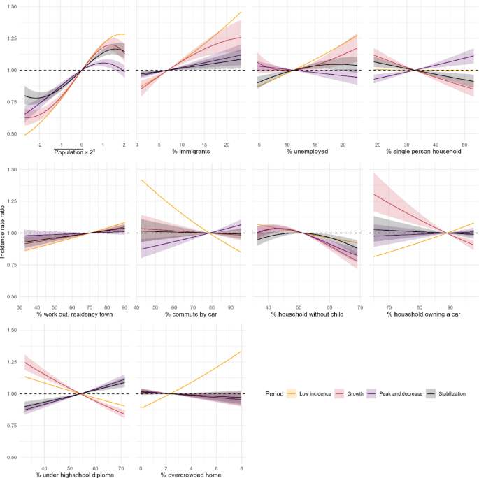
To assess the functional forms of the covariates, we used a penalized spline regression on the model M2 (covariates only) in each period, with a response following a negative binomial distribution. The estimation procedure in penalized spline regression12 provides the effective degrees of freedom (edf) for each covariate. This estimation and the graphical analysis of the corresponding functional forms were used to guide the choice of the degree of freedom used in the final models, implemented using orthogonal polynomials. The definitive degrees of freedom were selected empirically to maintain the most notable functional forms while not compromising the convergence of the Bayesian sampling procedure.
\(\beta\) parameters quantifying the association between the incidence rates of cases and the evaluated covariates were set to follow a centred normal prior distribution of variance 1000, and \({\tau }^{2}\) followed an Inverse-Gamma prior, with shape 0.1 and scale 1. The prior for \(\rho\) is set internally in the package as a uniform distribution in [0,1]. For each model fitting, 3 parallel Monte-Carlo Markov Chains were generated to produce 6,000 samples from the posterior distribution for each parameter. Convergence was assessed using Gelman plots and the potential scale reduction factor13. For the random effects’ parameters (\({\tau }^{2}, \rho\)) the median of the posterior distribution of the parameters was used as punctual estimate, and the credibility interval was built using the 2.5th and 97.5th centiles of the posterior distribution. The random variance \({\tau }^{2}\) is presented as a standard deviation \(\tau\), additive on the log-incidence scale and as \(\text{exp}\left(2\tau \right)\), multiplicative on the incidence scale. For the fixed effects of covariates, the estimated incidence rate ratios (IRR) for a covariate \(p\) were defined as the ratio between the predicted incidence rate at a given value of the covariate over the incidence rate at the mean value of the covariate, and plotted. The predicted IRR for each IRIS and period, using the overall mean predicted incidence rate as a denominator, was presented using cartography.
One major hypothesis in Poisson process modelling is that the probability of the next event is independent from the number of events which occurred previously. When modelling counts of cases aggregated over time as is the case in our study, this implies that the number of expected cases in one given IRIS is strictly proportional to the number of subjects at risk in this IRIS. For an infectious disease, this is not the case as the probability of contamination within one IRIS is a function of the number of contacts between residents and the number of infectious residents, which themselves may vary as a function of total population within this IRIS. To relax this hypothesis, models M2 and M4 include as a predictor the number of person-week centred on the mean person-week count per IRIS in the study region. The resulting IRR estimates the effect of the size of the population in a given IRIS upon the infection risk of an individual living in this IRIS.
Each model was evaluated by computing the Moran index of the residuals to assess whether the model was successful in accounting for the spatial autocorrelation, 1 indicating a complete positive autocorrelation and 0 no autocorrelation. We used the deviance explained to measure and compare, for each period, the goodness-of-fit of the models. The deviance explained by models M2, M3, and M4 compared to the null (M1) was used to assess the improvement in goodness-of-fit, with 1 indicating a perfect fit and 0 a fit no better than the null model. Predictive quality was evaluated using the quantile of the observed count of cases in the posterior predictive distribution of the counts for each unit. The observed value was classified in three categories: under the 5th or above the 95th quantile giving a poor prediction, under the 25th or above the 75th quantile giving a mediocre prediction, and within the interquartile range giving a satisfying prediction.
Detailed models’ specification, weight matrix computation, results from the edf determination (Figure S1) and evaluation of the MCMC sampling and of the priors’ influence (Figure S2) are reported in Supplementary Material. All analysis was conducted using R software (4.4.0). Travel times were computed using the Conveyal R5 routing engine14. Geographic data was extracted from the OpenStreetMap dataset. The model parameters were estimated using the package CARBayes15, and the functional form exploration was conducted using package mgcv.
The dataset of infection cases used in this study is composed of aggregated counts with censorship of statistical units for which there was between 1 and 5 observations. Therefore, we deemed the data anonymized16, with no further Institutional Review Board approval necessary under French law. The infection data collection in France was mandatory for the study period and a default authorization for the reuse of data for research purposes was included in the relevant law and subsequent decree2.