Mapping the regulatory genetic landscape of complex traits using a chicken advanced intercross line

Ethics approval

All animals involved in this study were housed and treated in accordance with the guidelines approved by the Animal Welfare Committee of Agrobiotechnology of China Agricultural University (Approval No. SKLAB-2014-06-07). Specifically, all animals were individually housed under controlled conditions (22 ± 2 °C, 50–60% humidity) with exposure to natural daylight and free access to feed and water. During the rearing period, qualified veterinary personnel conducted daily inspections and regularly monitored the chickens’ health and welfare, including assessments of physical appearance, behavior, feed and water intake. Any individuals exhibiting signs of abnormal health were promptly isolated and treated. At the end of the experiment, all chickens were euthanized by cervical dislocation performed by trained personnel. Death was confirmed by the cessation of respiration and heartbeat, as well as the absence of the corneal reflex.

Experimental population and phenotyping

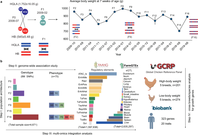
A large distant intercross pedigree was initiated in 2008 from two divergent chicken lines, high-quality chicken Line A (HQLA), a broiler line bred by Guangdong Wiz Agricultural Science and Technology, Co. (Guangzhou, China), and Huiyang Bearded chicken (HB), a native Chinese breed. The body weight of HB chickens at 7 weeks of age was, on average, less than one-third of those of HQLA (p −16). Detailed feeding regimes and F0 to F16 mating schemes have been described in Fig. 1 and earlier by Sheng and Wang et al.23,49.

The data of 75 traits were collected or processed in the F16 generation, including growth and development (GD, n = 36), tissue and carcass (TC, n = 23), feed intake and efficiency (FE, n = 9), blood biochemical (BB, n = 3) and feather characteristics (FC, n = 4) (Supplementary Data 2; Supplementary Note 2).

Similarly, we selected 21 phenotypes shared by F2, F9, and F16, and conducted a comparative analysis with F16 (Supplementary Data 14; Supplementary Note 3).

DNA extraction and Tn5 library construction

Blood samples were collected from the chickens at 5 weeks of age using the Laboratory-made FTA card. DNA was extracted from the blood samples using magnetic bead technology.

Equal amounts of Tn5ME-A/Tn5MErev and Tn5ME-B/Tn5MErev were incubated at 72 °C for 2 min and then placed on ice immediately for 1 min. Tn5 (Karolinska Institutet 171 77 Stockholm, Sweden) was loaded with the Tn5ME-A+rev and Tn5ME-B+rev in 2× Tn5 dialysis buffer at 25 °C for more than 2 h. All linker oligonucleotides were the same as those described in the previous report50.

Tagmentation was conducted at 55 °C for 10 min by mixing 4 μL 5×TAPS-MgCl2, 2 μL dimethylformamide (DMF) (Sigma Aldrich), 1 μL of the Tn5 pre-diluted to 16.5 ng/μL, 10 ng DNA (may be adjusted based on enzyme activity), and nuclease-free water. The total volume of the reaction was 20 μL. Subsequently, 3.5 μL 0.2% SDS was added, and Tn5 was inactivated for another 10 min at 55 °C.

KAPA HiFi HotStart ReadyMix (Roche) was used for PCR amplification by mixing 1 U HotStart DNA Polymerase, 10 μL 5× KAPA HiFi Fidelity Buffer, 2 μL dNTP Mix (10 mM each), 4 + 4 μL i5/i7 primers (5 μM) and 5.5 μL nuclease-free water. The PCR mix was added to the digestion products. The primers were designed for MGI sequencers, with the reverse primers containing different index adapters to distinguish individual libraries. We employed two index systems, one with 96 tags (P_1-96) and the other with 192 tags (C_1-192) to support future expansion. The PCR program was as follows: 9 min at 72 °C, 30 s at 98 °C, and then 9 cycles of 30 s at 98 °C, 30 s at 63 °C, followed by 3 min at 72 °C. The products were quantified using Qubit Fluorometric Quantitation (Invitrogen). The groups of 96 or 192 indexed samples were then pooled with equal amounts.

PCR products were size-selected and purified using the VAHTS DNA Clean Beads (Vazyme). The 0.8× and 1.3× sample volumes of DNA Clean Beads were used to remove most of the short and long fragments, respectively. The fragment sizes obtained via this method were ~300–900 bp, and the fragment size with the highest proportion was 500 bp. Final library quality (concentration and fragment size distribution) was determined using Qubit 4.0 (Qubit® dsDNA BR Assay Kit) and Qsep100, respectively. Sequencing was performed within 48 h after DNA cyclization and rolling circle amplification. All libraries were sequenced in one or two lanes of the MGISEQ-2000 to generate 2 × 100 bp paired-end reads (Supplementary Fig. 19a).

Sequencing and quality control

This study involved two types of sequencing libraries, namely typical whole-genome sequencing libraries (WGS, high coverage for F0 and 75 F16 samples, http://farmrefpanel.com/GCRP/#/, Supplementary Data 1) and Tn5-based low coverage sequencing libraries (LCS). For LCS, 4772 qualified libraries were sequenced using MGISEQ-2000 to generate 2 × 100 bp paired-end reads. The sequencing experiments were performed on the MGISEQ-2000 system at the National Research Facility for Phenotypic and Genotypic Analysis of Model Animals (Beijing) and State Key Laboratory of Animal Biotech Breeding. BCL files as primary sequencing output were converted into FASTQ files using bcl2fastq2 conversion software (version 2.16.0). The sequencing adapter was masked and trimmed during the conversion process. After the trimming step, the PE reads were subjected to a filtering process: SLIDINGWINDOW:4:15 and MINLEN:75 by Trimmomatic-0.36. The average percentage of the clean reads was 95%. The quality control check report of the filtered reads was generated using FastQC software (http://www.bioinformatics.babraham.ac.uk/projects/fastqc/). Next, we used a custom script to split each sample index and obtained 4772 samples. Of these, samples with a sequencing depth less than 0.1× of the chicken genome (1.06 Gb) and duplicate samples (IBS > 0.9) were removed. The remaining 4671 samples were retained for subsequent analysis.

Mapping and variant and variant callingWGS data SNP calling

We analyzed the high-depth sequencing data of 31 F0 founders, F16 samples, and other local chickens and commercial chickens using GTX (Supplementary Data 15). A commercially available FPGA-based hardware accelerator platform was used to map reads to the GRCg6a reference genome (Ensembl version 104) and variant calling. The alignment process was accelerated through the FPGA implementation of a parallel seed-and-extend approach based on the Smith-Waterman algorithm, whereas the variant calling process was accelerated via the FPGA implementation of GATK HaplotypeCaller (PairHMM)51. GATK multi-sample best practice52 was used to call and genotype SNPs for these samples, and the SNPs were hard filtered with a relatively strict option “QD  60.0||SOR > 3.0||MQRankSum 

LCS data SNP calling

For LCS data, the clean reads were mapped to the GRCg6a reference genome (Ensembl version 104) using BWA53. This was followed by read group addition, read pair sorting, marking duplicate reads, and building bam index by the Picard tools (http://broadinstitute.github.io/picard, v2.20.4). The indel realignment and base quality recalibration modules in GATK51 were applied to realign the reads around indel candidate loci and to recalibrate the base quality. The above steps are implemented in GTX-align, which is an FPGA-based hardware accelerator system (1–2 min/sample from clean FASTQ to BAM) on the high-performance computing platform of the State Key Laboratory of Agrobiotechnology. Variant calling was performed using the BaseVar and hard filtered with EAF ≥ 0.01 and the depth ≥ 1.5 times the interquartile range. The detailed BaseVar algorithm used to call SNP variants and to estimate allele frequency has been previously described54. We used STITCH55 (v1.1.2) to impute genotype probabilities for all individuals. The key parameter K (number of ancestral haplotypes) was set to 15. Raw SNPs were filtered with an imputation info score > 0.4, call rate > 0.95, and minor allele frequency (MAF) > 0.01. After filtering, 8,050,756 SNPs remained (Supplementary Fig. 19b). We utilized the SNPs from 108 samples, each of which simultaneously had both WGS and LCS data. We converted them to the 0/1/2 format and calculated the concordance between WGS and LCS data, defined as genotypic concordance; a higher concordance indicated a higher imputation accuracy of our LCS data. The SNPEff program56 was used to annotate variants.

RNA-seq library construction and sequencing data analysis

The total RNA of the duodenum and hypothalamus were extracted using TRIzol reagent (Invitrogen, Carlsbad, CA, USA) according to the manufacturer’s recommendations. To eliminate DNA contamination, all samples were treated with RNase-free DNase. The concentration and purity of the RNA samples were determined with a Nano Photometer spectrophotometer (Implen, CA, USA), and the RNA integrity number (RIN) of each RNA sample was determined using Agilent 4150 RNA (Agilent Technologies, CA, USA). cDNA synthesis was performed using a PrimerScript™ RT Reagent Kit (Takara, Dalian, China) according to the manufacturer’s instructions. Briefly, 1 μg of total RNA was mixed with DNA Eraser, and the mixture was incubated at 42 °C for 2 min on an EasyCycler® 96-well thermocycler (Analytik, Jena, Germany). Subsequently, oligo-d(T) primer, random hexamers, and dNTPs were added, and the mixture was incubated in a thermocycler at 37 °C for 15 min and 85 °C for 5 s.

The concentration and integrity of the were measured and checked for concentration and integrity using Nano Photometer spectrophotometer (IMPLEN, CA, USA) and an Agilent Bioanalyzer 4150 system (Agilent Technologies, CA, USA). The library was constructed using Hieff NGS Ultima Dual-mode mRNA Library Prep Kit for MGI (Yeasen Biotechnology, Shanghai, China) according to the manufacturer’s protocol. After library construction, the library was converted using the MGIEasy Universal DNA Library Preparation Reagent Kit (BGI, Shenzhen, China) for compatibility and sequenced on the DNBSE-QT7 platform (MGI). For quality control, we used fastp57 default parameters for filtering (v0.22.0). We aligned the clean reads to the GRCg6a reference genome (Ensembl version 104) using hisat258 (v2.2.1) with parameters of “–dta –new-summary -t -p 48 -x $index -1 $fq1 -2 $fq2.” Featurecounts.R of Rsubread (v2.12.0) was used for quantification, and edgeR (v3.40.0) was used for differential analysis.

Population structure analysis

ADMIXTURE59 (v1.3.0) was used for estimating an individual’s ancestry proportions from F0 and F15 genotype data (the F15 individuals were the paternal progenitors of all F16 samples). PCA was performed using Plink60 (v1.90) on the parental HB (n = 15), HQLA (n = 16) and 100 random samples from each of F2, F9, and F16. Vcftools61 (v0.1.17) was used to calculate allele frequency with the parameter “–freq2,” and nucleotide diversity analysis with the parameter “–window-pi 300000.” We used Plink60 (v1.90) with the parameters “–het” to calculate the inbreeding coefficient. We used PopLDdecay62 (v3.41) with parameters of “-MAF 0.01 -MaxDis” to perform LD decay analysis on different generations and use Plot_MultiPop.pl “-bin1 50 -bin2 1500 -break 500 -maxX 2000 -keepR” to draw. For haplotype diversity analysis, we used Plink60 (v1.90) with parameters of “–indep-pairwise 1000 kb 1 0.4” to filter LD on 4671 samples, resulting in 18,325 SNPs. We used five SNPs as windows to perform windowing and calculated each window haplotype type and the main effect haplotype frequency (the sum of the top four main effect haplotype frequencies).

GWAS and fine mapping

The heritability of the 75 phenotypes was calculated using a mixed linear model of GCTA63 (v1.93.3) with parameters “gcta64 –grm test –pheno pheno.txt –reml –out test”, corrected for batch and sex as covariates. We used GCTA63 (v1.93.3) with parameter “–reml-bivar” to calculate the genetic correlation between two phenotypes.

We simultaneously conducted GWAS on 75, 18, and 19 phenotypes of F16, F2, and F9, respectively (Supplementary Data 2, 6 and 14). First, we used GCTA63 (v1.93.3) with parameters “–make-grm” and “–grm-sparse” to construct the kinship and sparse matrices. Subsequently, we used a mixed linear model of fastGWA64 to perform GWAS.

$${{{\rm{y}}}}={{{{\rm{x}}}}}_{{{{\rm{snp}}}}}{{{{\rm{\beta }}}}}_{{{{\rm{snp}}}}}+{{{{\rm{X}}}}}_{{{{\rm{c}}}}}{{{{\rm{\beta }}}}}_{{{{\rm{c}}}}}+{{{\rm{g}}}}+{{{\rm{e}}}}$$

(1)

where y is an n × 1 vector of phenotypes; xsnp is a vector of mean-centered genotype values for the variant of interest, with its effect size βsnp; Xc is the incidence matrix of fixed covariates (sex and batch) with their corresponding coefficients βc; g is a vector of the total genetic effects captured by pedigree relatedness; e is a vector of residuals.

For the 75 and 19 phenotypes of the F16 and F9 generations, respectively, we first used the false discovery rate (FDR) for correction and selected SNPs with FDR 2, owing to the high LD between SNPs, SimpleM.R was first used to determine the number of independent SNPs; further, the initial QTL was determined based on Bonferroni 0.05 (p r2 

The heritability of the QTL was calculated using the GCTA63 bivariate GRM model with parameters “gcta64 –reml-bivar –mgrm multi_grm.txt –pheno test.phen”. We assessed the sharing of our detected QTLs with reported QTLs using the QTLdb database (https://www.animalgenome.org/cgi-bin/QTLdb/GG/index, Retrieved 28 December 2023), and if the QTLs of the two collections had overlapped, we considered the two to be shared.

We used Bedtools65 with “bedtools intersect” to annotate all QTLs for the 43 F16 phenotypes. For the QTL where a single gene was identified, we queried its gene function in mice according to the https://genealacart.genecards.org/ database and determined its relationship with growth and their development-related genes and corresponding QTLs.

Integrating eQTL and FAANG with GWAS

We integrated the eQTL data of 28 tissues from the chicken GTEx project and the FAANG annotation of 23 tissues from the chicken FAANG project with 40 F16 growth- and development-related phenotypes with significant GWAS signals to further identify functional genes (Supplementary Table 3). We utilized the GCTA63 bivariate GRM model for the calculation of heritability for each functionally annotated region and molQTL:

$${{{\rm{y}}}}={{{\rm{X}}}}{{{\rm{\beta }}}}+{{{\rm{g}}}}1+{{{\rm{g}}}}2+{{{\rm{e}}}}$$

(2)

where y is the phenotype, Xβ is the fixed effect (sex, batch); g1 is the genetic effect of functional annotation regions or molQTL; g2 is the genetic effect of all SNPs upstream and downstream of the functional region beyond 100 kb; e is a vector of residuals.

For the heritability obtained by “gcta64 –reml-bivar –mgrm multi_grm.txt –pheno test.phen –out test”, considering the different number of SNPs in each interval, we corrected for the number of SNPs and performed a log transformation.

For the growth and development-related phenotypes of the F16 generation that exhibited significant GWAS signals, we utilized all SNPs as a background for calculating enrichment and used a hypergeometric distribution test to calculate P values.

Enrichment factor = (target region significant SNPs/total significant SNPs)/(target region all SNPs/genome-wide total SNPs).

To assess whether eQTLs were significantly enriched among the notable GWAS variants, we used QTLEnrich (v2)10 to measure the enrichment degree between significant eQTLs and GWAS loci.

We performed single- and multi-tissue transcriptome-wide association studies (TWAS) using SPrediXcan66 and SMultiXcan67, which are parts of the MetaXcan (v0.6.11) framework. Briefly, we trained Nested Cross-Validated Elastic Net models with protein-coding genes and their corresponding SNPs within a 1 Mb cis-window across all 28 tissues. Predictive models with cross-validated correlation ρ > 0.1 and prediction performance p 

To investigate the pleiotropic association between molecular phenotypes and complex traits, we performed a Mendelian Randomization analysis using the SMR software68 (v1.3.1). This software enables the utilization of summary-level data from GWAS and eQTL studies. To configure the SMR software appropriately, the molQTL data generated by tensorQTL69 in this study was first converted into the BESD format using the options “–fastqtl-nominal-format –make-besd.” We then conducted the SMR test and applied multiple testing correction using the FDR approach. Gene-trait pairs with corrected p value 

To identify shared genetic variants between GWAS and eQTL, we conducted a colocalization analysis using fastENLOC70 (v2.0). First, we fine-mapped the putative causal variants for each eGene using a Bayesian multi-SNP genetic association analysis algorithm known as the deterministic approximation of posteriors (DAP), with the current version being DAP-G71 (v1.0.0). Using the DAP-G results, we generated a probabilistic annotation of molQTL using the “summarize_dap2enloc.pl” script. Next, we calculated approximate LD blocks with PLINK60 v1.9, using the options: “–blocks no-pheno-req –blocks-max-kb 1000 –make-founders”. The posterior inclusion probability (PIP) for GWAS loci was determined for each LD block using TORUS, with the options: “–load_zval -dump_pip”. By integrating GWAS PIP values, we performed the final colocalization analysis using the fastENLOC70 tool and obtained the gene variant-level colocalization probability (GRCP). GRCP > 0.1 was set as the significance threshold.

Identification of the major effect Q of GGA1 using outgroup data analysis

For the QTL of BW8 (GGA1:170,522,957–171,337,377), we sliding windowed the QTL according to 20 kb and obtained a total of 34 windows, screened the loci with p −16 in each window, calculated the frequency of each haplotype, and performed haplotype association analysis.

A haplotype-based association analysis was performed in each window using the model:

$${{{\rm{Y}}}}={{{\rm{X}}}}{{{\rm{\beta }}}}+{{{\rm{Zu}}}}+{{{\rm{e}}}}$$

(3)

where Y is a column vector representing the BW8 of the F16 individuals, and X is the design matrix that includes coding for chickens’ sex. For each specific interval, n haplotypes were constructed from m individuals based on several SNPs. Z is the design matrix (m × n) that contains the haplotype counts for each individual, coded as 0, 1, or 2. β is a vector estimating the fixed effect of sex, u is a column vector estimating the allele substitution effects for each haplotype, and e represents the normally distributed residual.

Similarly, we used low-body-weight chickens (HB, CH (Chahua), DWS (Daweishan), SY (Silkies), ZJ (Tibet)) and high-body-weight chickens (HQLA, CBA (commercial Broiler Line A), CBB (commercial Broiler Line B), KB (Cobb), YXB (White Plymouth Rock) and Red Junglefowl (RJF)) from GCRP (http://farmrefpanel.com/GCRP/#/, Supplementary Data 15) to calculate the frequencies of the corresponding haplotypes. Combined with the haplotype association analysis effect values, we determined q/Q; the frequency of high-body-weight chickens minus the low-body-weight chickens of the haplotype was greater than 0.2, and the haplotype was Q for increasing body weight and vice versa for the q haplotype. Combined with the annotations of the candidate functional genes in each window, a total of one q and four Q were identified.

Cross-species analysis

To evaluate the enrichment of genes linked to human traits and diseases in relation to five chicken growth traits (the functional genes identified exceeded 60), we collected GWAS summary statistics for 20 human complex traits from the UK Biobank and Yanglab (Supplementary Data 12 and 13). We mapped the functional genes in chickens to their corresponding human orthologous genes, including 1-1 orthologous, complex orthologous genes, based on the Ensembl database (v102). Subsequently, we conducted LD score regression analysis72 (https://github.com/bulik/ldsc). Heritability enrichment was determined by calculating the proportion of trait heritability attributed to SNPs within the specific annotation relative to the total number of SNPs in that annotation. Additionally, we investigated the impact of homologous human genes, identified from five chicken growth traits, on significant human phenotypes using the PheWAS database (https://atlas.ctglab.nl). Chicken and human SNP conversions were achieved using the UCSC liftover tool (https://genome.ucsc.edu/cgi-bin/hgLiftOver), and SNP annotations were obtained using SNPEff56.

Dual-luciferase reporter assay

For the candidate SNPs identified through GGA4 and GGA24 (Supplementary Table 4), we constructed a promoter vector (pGL3-basic luciferase reporter vector) and an enhancer vector (pGL3-enhancer luciferase reporter vector) to verify the transcriptional activity of the candidate SNPs on functional genes. The target sequence was centered on the candidate SNPs and extended 500 bp up and down. It was synthesized and cloned into the promoter or enhancer vector. DF-1 cells (chicken fibroblast cell line) were cultured in a Dulbecco’s modified Eagle medium (Gibco, USA) supplemented with 10% fetal bovine serum (Gibco, USA), 100 IU/mL penicillin, and 100 μg/mL streptomycin (Gibco, USA). Lipofectamine 3000 reagent (Invitrogen, USA) was used for transient transfection following the manufacturer’s protocols. The recombinant plasmid was transfected into the DF-1 cells together with the PRL-TK plasmid (Promega, USA). The DF-1 cells were then cultured in 24-well culture plates (Thermo Scientific, USA) at 37 °C and 5% CO2 for 48 h. Firefly and Renilla luciferase activities were measured at 48 h post-transfection using a Dual-Luciferase Assay System Kit (Promega, USA) according to the manufacturer’s instructions. Luminescence was detected using a microplate reader (Tecan, Switzerland), and firefly luciferase activities were normalized to Renilla luminescence in each well.

Real-time (RT) PCR experimental verification

Small intestine qRT-PCR was performed by using the SYBR Green Master Mix (Takara, Dalian, China) on Applied BiosystemsTM7300 qRT-PCR system (ABI, CA, USA) according to the manufacturer’s protocol. The data were analyzed by using the 2−ΔΔCT method. The chicken β-actin gene was used as the reference gene for normalization. The primers used for qRT-PCR are listed in Supplementary Table 5.

Reporting summary

Further information on research design is available in the Nature Portfolio Reporting Summary linked to this article.