Device
The device is depicted in Fig. 1. Detailed fabrication procedures are outlined in the Methods. This device comprises a superconducting half-wavelength coplanar-waveguide resonator coupled to a DQD formed by in-situ crystal-phase engineering in an InAs NW22,36,37,41. Figure 1a shows an optical microscopy image of the resonator, fabricated by dry-etching an approximately 10 nm thick NbTiN film, atop a SiO2 substrate39. The small thickness of the superconducting NbTiN renders the resonator resilient to in-plane magnetic fields38,39, and the narrow center conductor width, approximately 380 nm, combined with the large kinetic inductance of NbTiN, results in an impedance of 2.1 kΩ. This large impedance enhances the vacuum electric field fluctuation amplitude compared to standard 50 Ω-type resonators, thereby increasing the dipolar coupling to the TLS42.
Fig. 1: Superconducting resonator coupled to singlet-triplet two-level system (TLS) in a crystal-phase nanowire (NW).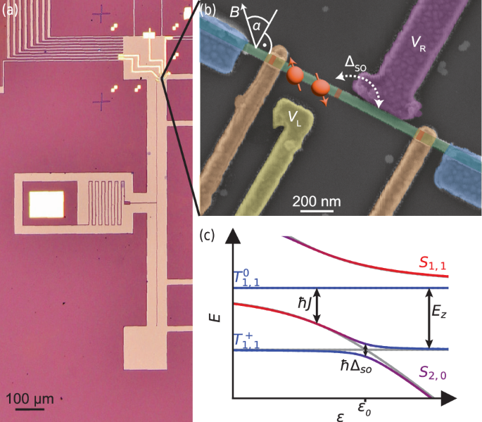
a Optical microscope image of the device showing a half-wave NbTiN resonator with a characteristic impedance of 2.1 kΩ. In the middle of the center conductor, a dc bias line is connected via a meandered inductor. b False-colored scanning electron micrograph of the crystal-phase NW device (image is rotated by − 90° with respect to a). The NW is placed at the position indicated in (a), and the purple gate line is galvanically connected to the resonator at its voltage anti-node. Tunnel barriers are highlighted in red. Using the gate voltages VL and VR, the device is operated with an even electron filling as depicted schematically. The spin-orbit gap ΔSO corresponds to the indicated spin-rotating tunnel transition, which forms the TLS. The in-plane magnetic field angle α is varied during the experiments using a vector magnet that controls the magnetic field B. c Level diagram for an even electron occupation as a function of the electrostatic detuning ε in the presence of strong SOI and finite magnetic field exhibiting singlet (S) and triplet (T) states. Subscripts denote the filling of the left and right dots, and the superscript denotes the spin quantum number of the triplet states (see methods). The avoided crossing between the spin-polarized triplet state T+ and the low-energy singlet state at ε = ε0 is detected using the resonator.
The TLS is formed by electronic states in a DQD, with tunnel barriers grown deterministically by controlling the InAs crystal phase during the vertical growth process of the NW36,37. The barriers are highlighted in the colored SEM image of Fig. 1b in red. The DQD forms within the zincblende segments of the NW, separated by wurtzite tunnel barriers. At finite magnetic fields and in an even electron configuration, the DQD states are singlet and triplet states, as depicted in the energy level diagram in Fig. 1c. The ground state and first excited state comprise a superposition of the spin-polarized triplet \(\left\vert {T}^{+}\right\rangle\), with an electron on each dot and the low-energy singlet state \(\left\vert {S}_{2,0}\right\rangle\), with two excess electrons on one dot and none on the other. As depicted in Fig. 1c, without spin-flip tunneling, the energy levels would cross at a detuning ε0 at which the Zeeman energy Ez equals the exchange energy ℏJ,
$${E}_{z}=\hslash J\approx \frac{\hslash }{2}\left({\varepsilon }_{0}+\sqrt{{\varepsilon }_{0}^{2}+4{t}_{c}^{2}}\right),$$
(1)
where tc is the inter-dot tunnel rate and ℏ denotes the reduced Planck constant. But the finite inter-dot tunnel coupling and a substantial Rashba-type SOI in the zincblende segments41 result in a spin rotation and in the hybridization of the original eigenstates, with an energy gap ℏΔso24. The two hybridized spin levels are split by a spin-orbit gap and constitute a spin-orbit-mediated electric dipole moment that couples to the electric field fluctuations of the resonator. This renders the resonator an effective probe for quantitative measurements of the TLS parameters.
Hybrid system at large magnetic fields
In our experiments, we measure the amplitude A and phase φ of a microwave probe tone transmitted through the resonator, capacitively coupled to the DQD. All measurements are performed at the mixing chamber plate of a dilution refrigerator with a base temperature of 70 mK. In Fig. 2a, the squared normalized transmission amplitude \({(A/{A}_{0})}^{2}\) through the resonator is plotted as a function of the probe frequency ωp with the DQD tuned into Coulomb blockade, rendering it irrelevant for the measurement. This figure displays probe frequency scans at magnetic-field amplitudes ∣B∣ = 0 mT and ∣B∣ = 100 mT, where the field is applied in-plane. As visible in Fig. 2(a), the transmission through the resonator recorded for ∣B∣ = 0 mT and ∣B∣ = 100 mT does not show any variation, demonstrating that the resonator remains unaffected for the magnetic fields used in our experiments.
Fig. 2: Characterization of the hybrid device.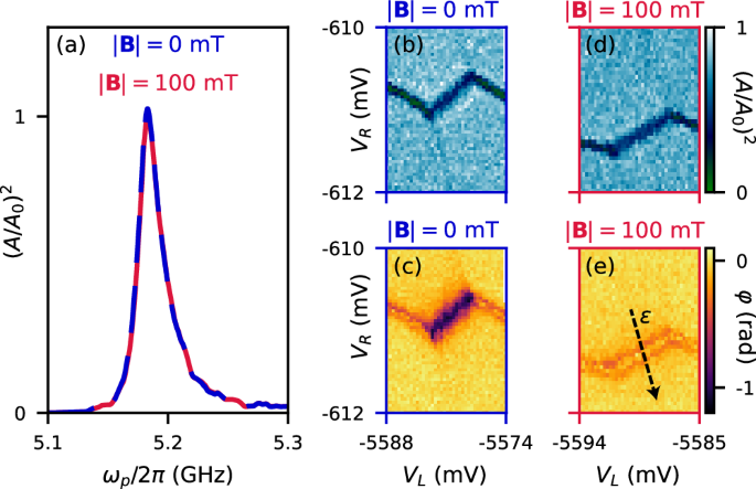
a Resonator transmission \({(A/{A}_{0})}^{2}\) as function of probe frequency ωp. Fits to a Lorentzian result in the resonance frequency ω0/2π = 5.1854 ± 0.0002 GHz, and decay rate κ/2π = 21.2 ± 0.4 MHz independent of the magnetic-field amplitude ∣B∣. The magnetic-field resilience of the resonator enables resonator-based investigation of the double-quantum dot (DQD). b–e Transmission \({(A/{A}_{0})}^{2}\) and phase φ close to resonance frequency as a function of gate voltages VL and VR applied to the DQD as illustrated in Fig. 1(b) at zero field and at ∣B∣ = 100 mT. Position and shape of the observed inter-dot transition signal vary as a function of ∣B∣ due to an interaction of the resonator with spinful DQD levels. In the remainder of the manuscript, the DQD detuning ε is varied by applying VL and VR along the arrow indicated in (e).
We now prepare the DQD in an even charge state22,43,44,45 and measure the resonator transmission at a frequency close to resonance. Figure 2b–e depict the transmission amplitude and phase as functions of the gate voltages VL and VR for in-plane field amplitudes of ∣B∣ = 0 and ∣B∣ = 100 mT.
Due to the electric-dipolar coupling between the resonator and the DQD, the resonator transmission directly reveals the charge stability diagram of the DQD46. At the inter-dot transition (IDT), the Zeeman energy and the exchange energy are degenerate (see Eq. (1)) and the hybridized states couple to the resonator. The IDT can be easily identified, signaled by lines with positive slopes in Fig. 2e.
Both, the position of the IDT in the gate-versus-gate map and the resonator response near the IDT strongly depend on the external magnetic field strength. This susceptibility to magnetic fields arises from the spin-dependent DQD transitions. In the following, we probe the resonator response as a function of electrostatic detuning ε, which is manipulated by varying the gate voltages VL and VR along the line indicated in Fig. 2e.
A double sweet spot
The main result of our work is represented by the dependence of the IDT characteristics on the in-plane field orientation. For this we show in Fig. 3a the resonator transmission phase φ close to the resonance frequency, plotted as a function of the in-plane angle α between the NW axis and the magnetic field, illustrated in Fig. 1b and Fig. 3b, and versus the electrostatic DQD detuning ε as defined in Fig. 2e. Similar data for varying magnetic field strength is shown in the SM. Figure 3a reveals that the detuning ε0, at which the IDT is observed, varies as a function of α. This angle dependence can be understood qualitatively by recognizing that the SOI introduces an anisotropic g-tensor and hence determines the Zeeman energy EZ and, according to Eq. (1), the position of the IDT ε0. Furthermore, the phase signal as a function of ε changes continuously from a negative shift in φ at α ≈ π/2 [3π/2] to a double-dip structure at α ≈ π [2π], because the SOI renders the magnitude of ΔSO and the dephasing rate γ angle-dependent by affecting the overlap of the spin wavefunctions24,30,40,47. For example, at α ≈ π/2, Δso > ω0, resulting in a dispersive resonator signal. In contrast, at α ≈ π, Δso ω0 so that an (avoided) crossing between the singlet-triplet TLS and the resonator is observed as function of ε. This crossing experimentally results in a double dip structure in the φ(ε) dependence, framing a positive shift at the center of the IDT, at ε ≈ ε0.
Fig. 3: Two-level system (TLS) parameters as a function of in-plane field angle at ∣B∣ = 100 mT.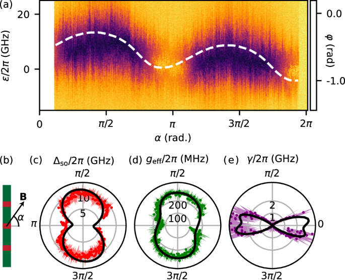
a Phase of the resonator transmission φ as function of electrostatic detuning ε and in-plane magnetic field angle α. The detuning ε, was calculated from the applied voltages, using the gate-to-dot lever arms (see Table 1). The dashed curve corresponds to the position of the inter-dot transition in the theoretical model, ε = ε0, to which a linear trend was added accounting for a drift of the gate voltage. b Schematic showing the alignment of the magnetic field B with respect to the nanowire (NW), where the NW color scheme represents the crystal-phase structure according to Fig. 1b. c Spin-orbit gap Δso as function of α. d Coupling strength geff between the TLS and the resonator as function of α. e TLS dephasing rate γ as function of α. When the field is parallel to the NW, α = ± π/2, a compromise-free sweet spot is found where maximal TLS transition frequency and coupling strength coincide with minimal total dephasing rate. c–e are extracted using input-output theory. The streaks symbolize the uncertainty of the fit. This uncertainty is a consequence of the uncertainty of the gate lever arms, which forms the most significant source of uncertainty in our experiment and is stated in the caption of Table 1. All curves overlaid on the data result from the theoretical model described in the main text, using a single set of fit parameters. During the measurement, a charge relocation occurred at a magnetic-field angle α ~1.9π resulting in missing data for α ∈ [0, 0.1π] ∪ [0.19π, 2π) in all subfigures.
Using input-output theory48 as described in the Methods, we extract the SOI gap Δso, the TLS dephasing rate γ, as well as the effective spin-photon coupling strength geff from the dependence of the resonator phase and amplitude on ε. The results are plotted as a function of in-plane angle α in Fig. 3c–e.
Excitingly, we find that, while Δso and geff are correlated with each other, they are anticorrelated with γ. In particular, when applying the magnetic field parallel to the NW, a compromise-free sweet spot is found, for which the spin-photon coupling strength geff is maximal while γ is minimal. To robustly estimate the spin-photon coupling and the dephasing rate at the sweet spot, we average over all extracted values in the interval α ∈ [55°, 125°] ∪ [235°, 305°] and find 〈geff〉/2π = 250 ± 15(30) MHz and 〈γ〉/2π = 11 ± 20(400) MHz, where the error corresponds to the statistical (systematic) uncertainty. Here, the large systematic uncertainty originates from the uncertainty of the gate lever arms stated in the caption of Table 1.
Theoretical description
In this section, we outline how the effective Hamiltonian yields the dashed white and solid black curves shown in Fig. 3a, c, and d. The consecutive section describes how the decoherence is modeled (black curve in Fig. 3e).
All curves are the result of numerically diagonalizing the Hamiltonian H5 in Eq. (12) in the Methods that describes the DQD states in proximity to the IDT. Thereby, we take into account an anisotropic g-tensor, identical for both dots, and a spin-orbit vector that is not aligned with the principal axes of the g-tensor. We point out that all curves are obtained from a single set of fit parameter, given in Table 1. The Landé g-factor varies between g = 10.5 and g = 5.25, depending on the field direction. And, taking into account the distance of the two quantum dots, d = 330 nm, the spin-orbit length is found as lso = 130 nm. These values are consistent with previous experiments9,49. In Methods Section V C, we describe the DQD model in detail and visualize the g-tensor based on the fitted parameters.
After finding the eigenenergies and eigenstates from diagonalizing the Hamiltonian H5, we focus on the ground state \(\left\vert 0\right\rangle\) and first excited state \(\left\vert 1\right\rangle\) with their respective energies E0 and E1. These states possess an electric dipole moment which is sensed by the resonator. Because Eq. (1) is only valid for small SOI, which is not the case for certain field alignments, we more generally determine the detuning ε0, at which the anti-crossing occurs, by identifying the minimum gap for which
$${\partial }_{\varepsilon }({E}_{1}-{E}_{0})=0.$$
(2)
The numerical solution for ε0 is plotted in Fig. 3a on top of the data (white dashed curve). The variations of the detuning ε0 of the IDT as function of α is caused by the g-tensor anisotropy. According to Eq. (1), this results in a variation of ε0 at which the Zeeman energy equals the exchange energy. As a consequence, the detuning ε0 at which the IDT is observed varies with the g-factor, which in turn is given by the field orientation. Then, we numerically calculate the SOI gap
$${\Delta }_{{{{\rm{so}}}}}={E}_{1}({\varepsilon }_{0})-{E}_{0}({\varepsilon }_{0})\,,$$
(3)
plotted as solid black curve in Fig. 3c. The variation of the SOI gap Δso is a consequence of the magnetic field orientation with respect to the anisotropic g-tensor and the spin-orbit vector. To calculate the vacuum Rabi coupling strength geff, we assume that the resonator couples to the electric dipole moment of the singlet-triplet TLS via the resonator vacuum fluctuations in the detuning of amplitude δε0 according to Eq. (11) in the Methods. This gives rise to the dipolar coupling strength as the vacuum Rabi rate
$${g}_{{{{\rm{eff}}}}}=\delta {\varepsilon }_{0}| \left\langle 0\right\vert {h}_{\delta \varepsilon }\left\vert 1\right\rangle |$$
(4)
plotted as solid black curve in Fig. 3d. Here, hδε is the operator describing small variations of the detuning, given by Eq. (15) in the Methods and evaluated at the center of the IDT, ε = ε0.
Decoherence
In the experiment, using input-output theory, we utilize the resonator as a probe to extract the total TLS dephasing rate γ, which is plotted in Fig. 3e, and defined by
$$\gamma =\frac{{\gamma }_{1}}{2}+{\gamma }_{\varphi },$$
(5)
where γ1 is the relaxation rate and γφ the pure dephasing rate. The primary sources of decoherence in quantum dots are typically hyperfine-interaction induced dephasing from atomic nuclei50,51,52, charge noise-induced dephasing33,34,53,54, or relaxation due to phonons55,56,57,58,59,60,61,62,63.
From our experiments, we extract an unexpected anti-correlation between the spin-photon coupling strength geff and the dephasing rate γ. Using our theoretical description, and Bloch-Redfield theory56,60,64, we investigate various possible decoherence mechanisms as outlined in the Supplementary Note 2. We find that consideration of magnetic noise stemming from nuclear spins or charge-noise due to phonons leads to the correct trend of γ as a function of the in-plane magnetic-field angle α. However, because we identify dephasing rates comparable to the maximum of γ(α) also for a charge qubit at a zero magnetic field, where magnetic noise is irrelevant, we hypothesize that phonons form the dominant noise source in our experiment. Therefore, here, we focus on phonon-mediated decoherence.
Figure 3e and Fig. 4a show the phonon-mediated relaxation \({\gamma }_{1}^{{{{\rm{ph}}}}}(\alpha )\) as a function of the in-plane field angle α overlaid on the measured dephasing rate γ. Considering only the effect of a single gapless, low-energy phonon band gives rise to the analytical functional dependence \({\gamma }_{1}^{{{{\rm{ph}}}}}(\omega )\) as function of phonon frequency, ω. Here, the longitudinal phonon modes couple to the detuning and tunneling through variations in the electrostatic potential due to their deformational interactions. This coupling leads to TLS relaxation (see Supplementary Note 2 for the derivation).
Fig. 4: Phonons as possible decoherence source.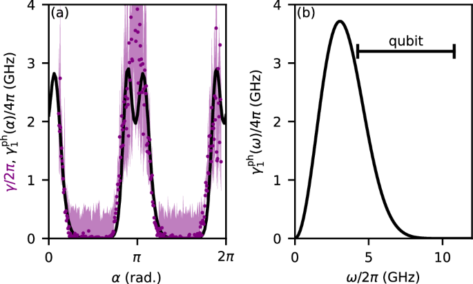
a Measured dephasing rate γ as a function of in-plane angle α (purple). The experimental data is plotted as purple points, and the error bar is given by a purple stripe. The error bars are dominated by the error associated with the gate-lever arm uncertainty. The black curve is the numerically calculated relaxation rate \({\gamma }_{1}^{{{{\rm{ph}}}}}(\alpha )\) originating from deformational phonons (see Section Decoherence). b Analytical relaxation rate \({\gamma }_{1}^{{{{\rm{ph}}}}}(\omega )\) as function of phonon frequency ω (see Equation (27) in Supplementary for details). The TLS operates in the frequency range as indicated with a negative slope of \({\gamma }_{1}^{{{{\rm{ph}}}}}(\omega )\). This explains the anti-correlation between the SOI gap Δso and the dephasing rate γ – a possible reason for the compromise-free sweet spot formation.
This dependence is plotted in Fig. 4b. These phonons lead to relaxation when their frequency is close to the TLS transition frequency ω ≈ Δso. Because the phonon-mediated relaxation is maximal when the phonon wavelength is comparable to the size of the dots at ω ≈ ωc, an increase in Δso leads to a decrease in \({\gamma }_{1}^{{{{\rm{ph}}}}}\). Therefore, a change in Δso as function of α results in the observed variations of \({\gamma }_{{{{\rm{1}}}}}^{{{{\rm{ph}}}}}\). In addition, variations of α result in a change of the electron-phonon coupling strength that enhances this effect and is considered in \({\gamma }_{{{{\rm{1}}}}}^{{{{\rm{ph}}}}}(\alpha )\), plotted as black curve on top of the data in Fig. 4a.
In Supplementary Note 2, we discuss magnetic noise. Additionally, in the Supplementary Note 2, we discuss 1/f-charge noise, which does not capture the functional dependence of γ as a function of the in-plane magnetic field angle α.