Mutually coherent DCR with 1-nm-precision
The interferometric DCR principle is rooted in the Fourier transform relationship, that a temporal shift τd corresponds to a linear phase of ωτd in the frequency domain (ω = mωr, where m is the comb line number with respect to the pump and ωr is the angular repetition rate). By measuring the multi-heterodyne phases for the signal and reference arms, denoted as ϕsig(ω) and ϕref(ω) in Fig. 1a, we can derive τd and distance L as,
$$L=c{\tau }_{d}/2=c\Delta ({\phi }_{{{{{\rm{sig}}}}}}(\omega )-{\phi }_{{{{{\rm{ref}}}}}}(\omega ))/2\Delta \omega .$$
(1)
The time-of-flight τd can be determined by linearly fitting ϕsig(ω) − ϕref(ω) in the frequency domain. Conversely, ref. 10 derived the time-of-flight by locating the RF pulse peaks in the time domain. Here, we refer to these two approaches as fToF and tToF, respectively. For fToF, high mutual coherence and stable ϕsig, ϕref are the keys for precise DCR. Note that we omit the influence of the air group index and treat the pulse group velocity as the vacuum light velocity c. This group index impact can be included by using two-color measurements33.
Fig. 1: Coherent dual-comb ranging (DCR) using counter-propagating (CP) solitons.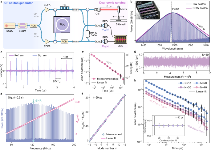
a Experimental setup for the CP solitons generation and DCR. ECDL external cavity diode laser, SSBM single-sideband modulator, AOM acoustooptical modulator, FBG fiber Bragg grating, EDFA erbium-doped fiber amplifier, PC polarization controller, Col collimator, BPD balanced photodetector, IM intensity modulator, PM phase modulator, VOA variable optical attenuator. b Optical spectra of the CP solitons. The inset shows the nanophotonic chip. c Dual-comb inteferogram in the signal and reference arms. d Power spectrum of the signal arm and the corresponding phase spectrum. e Allan deviation of phase different between the 4th and the 9th lines. f Phase difference between the signal and the reference arms measured in 50 μs. g Fitting the phase difference in panel (f) yields the distance over 104 time slots. h DCR Allan deviation when selecting different number of comb lines for fitting, all showing t−1/2 scaling. The inset shows all the selections yield the same distance, but with different standard deviation (see error bars).
Our setup to generate CP solitons with VFL is shown in Fig. 1a, see Methods. Optical spectra of the CP soliton microcombs are plotted in Fig. 1b. One of the microcombs was sent to and reflected from a cooperative target (a mirror) to heterodyne beat with the other microcomb to generate the DCR signals. The dual-comb inteferogram was registered by balanced photodetectors (BPDs) and digitized by an oscilloscope (see “Methods” for details). An example of the interferogram with δfr = 1.62 MHz is shown in Fig. 1c. We then Fourier transform the RF pulses to have the power spectrum and ϕsig(ω) shown in Fig. 1d. Mutual coherence enables direct transform without any digital correction as needed in many cases3, which can greatly relax computation burden in future PIC-based DCR systems. A power rSNR (signal over average noise floor) exceeding 80 dB can be obtained within a measurement time t = 0.5 s. To show the phase stability between the CP solitons, we plot the Allan deviation of ϕsig(9ωr) − ϕsig(4ωr) in Fig. 1e, which scales as t−1/2 and reaches 0.5 mrad at 0.1 s. The relative timing stability between CP solitons can be estimated as (ϕsig(9ωr) − ϕsig(4ωr))/5ωr, reaching 0.1 fs at 0.1 s.
Then, we analyze ϕsig − ϕref using RF pulses measured within 50 μs and observe an excellent linearity for the used N = 30 lines (excluding the pump, see Fig. 1f). Fitting the relative phase yields the distance in multiple 50 μs slots (Fig. 1g). The DCR precision is evaluated by Allan deviation and shows a t−1/2 scaling with a normalized precision of 0.6 nm\(\cdot \sqrt{{{{{\rm{s}}}}}}\) (Fig. 1h). The normalization does not include the information of absolute distance. The distance from the collimator to the target is about 13 cm (fiber length from the collimator to the signal BPD is about 3 m), when evaluating this precision. We further changed the used comb line number from N = 30 to other numbers to evaluate the precision. Normalized precision as high as 0.5 nm\(\cdot \sqrt{{{{{\rm{s}}}}}}\) (reaching 1.1-nm-precision at 0.2 s) is possible for our system. The precision is reached by pure fTOF without using interferometric phase of a carrier frequency2. The inset of Fig. 1h confirms that our measurement always yields the same distance when using different comb line number N.
Precision of DCR
Theoretically, the DCR precision is derived as (see “Methods”),
$$\sigma=\frac{\sqrt{3}\sqrt{1+\alpha }c}{N{\omega }_{r}\sqrt{N}\sqrt{{{{{{\rm{rSNR}}}}}}_{{{{{\rm{eff}}}}}}}}=\frac{\sqrt{3}\sqrt{1+\alpha }c}{2\pi B\sqrt{N}\sqrt{{{{{{\rm{rSNR}}}}}}_{{{{{\rm{eff}}}}}}}},$$
(2)
where rSNReff is the effective rSNR for the signal arm, B = Nfr is the used comb bandwidth, and α is the ratio between the rSNReff in the reference and the signal arms. rSNR(m) is defined as the RF power ratio between the mth line and the average noise floor (see Fig. 1d for illustration). Note that rSNR is defined in the frequency domain and differs from the ranging signal-to-noise ratio used in ref. 4. The relationship between rSNReff and rSNR(m) is discussed in Methods and Supplementary Fig. 1. The phase of a measured RF tone has contribution from both the signal and noise (inset of Fig. 2a). Thus, the phase deviation of a measured RF line (σϕ) is determined by the rSNR determines as,
$${\sigma }_{\phi }(m,t)=\frac{1}{\sqrt{{{{{\rm{rSNR}}}}}(m,t)}}.$$
(3)
σϕ(4, t) plotted in Fig. 2a confirms this relationship. σϕ(m, t) for other comb lines also support Eq. (3) (Supplementary Fig. 3). σϕ divided by 2πB yields the timing (thus, distance) deviation. The \(1/\sqrt{N}\) term is added as fitting multiple points leads to higher stability34 (Supplementary Note 1). To verify it, we analyzed the DCR precision for a fixed B = 3.2 THz but selecting lines with different spacings (thus, different N). A \(1/\sqrt{N}\) scaling is observed for the normalized precision (Fig. 2b). Finally, α is included as the DCR signal is derived from the phase difference between the signal and reference arms (Eq. (1)).
Fig. 2: Measurement precision of DCR.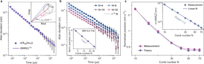
a Allan deviation of the phase of the 4th comb line, which equals 1/\(\sqrt{{{{{\rm{rSNR}}}}}}\). The inset shows an illustration of the relationship between rSNR and phase deviation. b DCR precision for a fixed comb bandwidth B = 3.2 THz, but selecting comb lines with different spacing (thus, different used comb line number N). The inset shows the normalized precision improves as N−1/2. c Measured DCR precision agrees with the theoretical precision determined by Eq. (2). The inset confirms the N−3/2 trend in our theory.
Our measured DCR precision is in excellent agreement with the theory (Fig. 2c). The precision no longer improves evidently for N > 40. This is because rSNR(m) decreases for large ∣m∣, resulting in a reduced rSNReff. We numerically calculated rSNReff based on rSNR(m) of the used microcomb lines (see “Methods” and Supplementary Fig. 1 for details). After taking the decrease of rSNReff into account, a scaling of N−3/2 is observed (see Eq. (2) and inset of Fig. 2b).
Therefore, the high DCR precision in our system can be attributed to the high rSNR and broad usable bandwidth. rSNReff can be further written as,
$${{{{{\rm{rSNR}}}}}}_{{{{{\rm{eff}}}}}}=\frac{K(B)}{{N}^{2}}\frac{{P}_{{{{{\rm{LO}}}}}}{P}_{{{{{\rm{sig}}}}}}}{{S}_{{{{{\rm{n}}}\,}}}{f}_{{{{{\rm{BW}}}}}}}=\frac{K(B)}{{N}^{2}}\frac{{f}_{r}^{2}{E}_{{{{{\rm{LO}}}}}}{E}_{{{{{\rm{sig}}}}}}t}{{S}_{{{{{\rm{n}}}}}}},$$
(4)
where Sn is the spectral power density of the RF noise floor, and fBW = 1/t is the resolution bandwidth; Psig(LO) and Esig(LO) are the received signal (local) optical comb power and energy, respectively; K(B) is a conversion coefficient that includes response from the BPD and variation of rSNR(m) within the used bandwidth. By combining Eq. (2) and Eq. (4), we have the DCR precision as,
$$\sigma=\frac{\sqrt{3K(B)(1+\alpha ){S}_{{{{{\rm{n}}}}}}}\sqrt{N}c}{2\pi B\sqrt{{P}_{{{{{\rm{LO}}}}}}{P}_{{{{{\rm{sig}}}}}}t}}=\frac{\sqrt{3K(B)(1+\alpha ){S}_{{{{{\rm{n}}}}}}}\sqrt{N}c}{{\omega }_{r}B\sqrt{{E}_{{{{{\rm{LO}}}}}}{E}_{{{{{\rm{sig}}}}}}t}}.$$
(5)
It can be seen that σ is proportional to \(\sqrt{N}\) for a given bandwidth B and comb powers. The comb power is ultimately limited by the saturation of the BPDs. Thus, small comb line numbers for microcombs are beneficial for enhancing DCR precision, but at penalty of a shorter non-ambiguity range due to the large line spacing ωr. The non-ambiguity range can be extended by swapping the signal and local combs for measurements2,10.
DCR with intensity loss or noise
Due to small N, only low comb power and pulse energy are needed for precise DCR when using microcombs (Eqs. (2), (5)). In experiments, we adjusted the loss in the signal arm (Fig. 1a) to measure DCR precision under different received powers. When reducing the power to 7 pW (attenuated by 67 dB), the dual-comb interferogram is already buried in the noise (Fig. 3a). However, an RF comb with rSNR over 10 dB can still be obtained after coherently averaging 0.5 s data (Fig. 3b). Mutual coherence for VFL solitons is the key to coherent averaging and resolving these RF tones. The low power measurement suggests our system can also work for non-cooperative targets.
Fig. 3: DCR with low received power and strong intensity noise.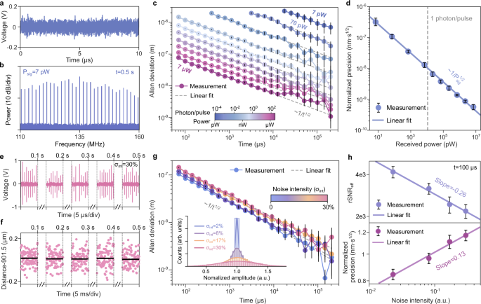
a Dual-comb interferogram signal with a received power of 7 pW. b RF spectrum of the signal in panel (a) after t = 0.5 s coherent averaging. c DCR Allan deviation of a series of received powers, all exhibiting t−1/2 scaling. d Normalized DCR precision, showing an inverse square-root relationship with the received power. e Measured RF pulses have randomly fluctuating amplitudes when introducing intensity noise on the received microcomb. f Measured distance in five 5 ms slots separated by 0.1 s (50 μs per measurement point) and solid lines are the average distance. g DCR Allan deviation under different intensity noise. The inset shows the distribution of the RF pulse amplitude. In the absence of intensity noise, the amplitude has a 2% fluctuation. The added intensity noise can introduce 30% amplitude fluctuation. h Deterioration of the rSNR under different intensity noise, which results in the increase of the DCR Allan deviation. The error bars in panel (d, h) correspond to the standard deviation in multiple measurements.
The DCR Allan deviation still scales as t−1/2, but with a lower normalized precision of 300 nm\(\cdot \sqrt{{{{{\rm{s}}}}}}\) (top curve in Fig. 3c). It means a micron-precision can be obtained in 0.1 s using a microcomb with 5.5 × 10⁻⁴ photon per pulse. Although a single microcavity soliton has an extremely low photon number, the total photon number used in 0.1 s is 5.5 × 10⁶ considering its 100 GHz repetition rate. The Allan deviation for a series of received powers is plotted in Fig. 3c, all exhibiting t−1/2 scaling. The normalized DCR precision decreases with the received power in a square-root trend, consistent with Eqs. (2), (5) (Fig. 3d).
Since the fToF-DCR relies upon optical phase measurements, our system is immune against intensity fluctuations. To showcase this feature, we inserted an intensity modulator (IM) and drove it by a broadband noise in the signal arm (Fig. 1a). The measured RF pulses have strong fluctuations in the amplitude (Fig. 3e). Despite these fluctuations, the measured average distance remains the same for five 5 ms slots separated by 0.1 s (t = 50 μs for a single data point, see Fig. 3f). The distribution of the normalized RF pulse amplitudes (normalized by the average amplitude) subject to different intensity noise levels is shown in the inset of Fig. 3g; the blue one is the case without IM noise. We used the standard deviation σint of this distribution to quantify the noise level. The added intensity noise can cause the RF pulses to have a 30% intensity fluctuation (see the labeled σint in the inset). DCR Allan deviation retains the t−1/2 scaling in the presence of the intensity noise (Fig. 3g, average received power is 15 μW). Nanometer-scale precision is still possible with σint=30%.
The Allan deviation does increase with σint, as the intensity noise reduces rSNR. rSNReff for the used 30 lines decreases with a slope of −0.26 in a log-log plot versus σint, while the change of the DCR Allan deviation has a slope of 0.13 (Fig. 3h). Such a −0.5 relationship between them further strengthens our theory in Eq. (2). Note that the rSNR reduction does not impact the DCR measured distance (Fig. 3f); it only means a longer measurement time is needed to reach a desired precision. The influence of intensity noise on ranging precision has also been evaluated for the dispersive interferometry technique using microcombs (see Supplement in ref. 26). Measurements and analyses therein exhibit a ~1 slope for ranging precision versus intensity noise, much larger than the 0.13 slope observed in Fig. 3h. We also used the RF pulse peak position for ranging (tToF-DCR), and intensity noise was observed to impact ranging precision stronger (see Supplementary Fig. 5). Supplementary Fig. 5 also suggests the decrease of rSNR in Fig. 3h mainly results from the reduction of the average received power caused by larger noise added to the IM. Although heterodyne detection was used in chaotic ranging in ref. 27, intensity cross-correlation was used for ranging, and intensity noise should also impact the measurement precision. The low intensity noise susceptibility can be useful when the measured target surface has varying reflection coefficients and may be used to distinguish amplitude and phase fluctuations induced by air turbulence35.
Near-Megahertz-DCV measurements
The high rSNR also enables DCR using a single-frame interferogram at a rate of δfr = 1.83 MHz, i.e., DCV at a rate up to δfr/2. Similar single-frame DCR was demonstrated in ref. 9, but optical power amplification was used. Here, we implement it without optical amplification. We experimentally inserted a phase-modulator (PM) into the signal arm (Fig. 1a). By driving the PM with sine-waves, the optical path length for the signal microcomb vibrates periodically. Figure 4a shows the DCR-measured optical path length change with a ~1 μm amplitude at update rates of 125 kHz and 1.83 MHz, when driving the PM at frequencies of 20 and 900 kHz, respectively. The measured distance changes follow the sine-drive signals (Fig. 4a). Data points appear sparse for the 900 kHz phase modulation, which was measured at a update rate of 1.83 MHz. However, the measurement still satisfies the Nyquist-Shannon sampling theorem.
Fig. 4: Near Megahertz dual-comb vibration (DCV) measurements.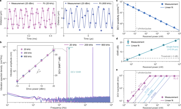
a Measured distance change with drive frequencies of 20 or 900 kHz. The received microcomb power was about 35 μW. b DCV spectra measured at three drive frequencies, all yielding sharp peaks with a high signal-to-noise ratio (SNR). The inset shows the measured vibration amplitude versus the drive power of the phase modulator (PM). c The DCV sensitivity (determined by the noise floor in panel (b) scales in a square-root way with the received microcomb power. d Deduced rSNR for a single-frame inteferogram under different received powers. This rSNR should exceed 3 dB for a reliable DCV measurement. The error bars correspond to the standard deviation in multiple measurements. e The highest vibration frequency that can be measured with different received powers. Below 200 nW power, the highest frequency decreases linearly with the power. When the comb line number becomes larger for a fixed total power, DCV at δfr/2 will need a higher received power.
Then, we analyzed the DCR-measured distance change in the frequency domain. A Blackman window was included to minimize spectral leakage in fast Fourier transform (FFT) in this analysis. In the frequency domain, the measured distance changes correspond to sharp peaks at 20, 200 and 900 kHz as shown in Fig. 4b (drive frequency at 200 kHz was also measured). The corresponding peak intensities are the same for all the three drive frequencies and are about 66 dB higher than the average noise floor. When varying the drive power from −10 to 20 dBm for the PM, we observed the peak amplitude scales in a square-root way with the drive power for all the three drive frequencies (inset of Fig. 4b). Such a relationship verifies the high accuracy of our DCV measurements.
The noise floor for the power spectral density in Fig. 4b provides a measure of the DCV sensitivity. We summarize this sensitivity versus received powers in Fig. 4c. For a nearly white noise floor, its noise spectral amplitude density has a linear relationship with the Allan deviation in DCR36. Since the DCR precision has an inverse square-root relationship with the received power (Fig. 3d and Eqs. (2), (4)), the measured DCV sensitivity also follows an inverse square-root scaling with the received power, and reaches a sensitivity of 0.4 nm/\(\sqrt{{{{{\rm{Hz}}}}}}\) (Fig. 4c).
To measure vibration at δfr/2, the received power should guarantee a sufficient rSNR(m, 1/δfr) for single-interferogram DCR. It is technically challenging to quantify rSNR(m, 1/δfr) directly, as fBW = δfr for a single-interferogram measurement. In practice, we derive it from rSNR at t = 100 μs, using the relationship that rSNR scales linearly with t for VFL solitons16. The minimum rSNR(m, 1/δfr) among the used 30 lines under different received powers is plotted in Fig. 4d. Our data process practice suggests that the minimum rSNR(m, 1/δfr) should exceed 3 dB to enable a reliable measurement. The received power needed to reach this threshold is about 100 nW (about 10 photon per pulse). For lower powers, we need to average longer time to reach the required rSNR, and the needed time t increases linearly with decreasing Psig (Fig. 4e). Therefore, the highest vibration frequency decreases linearly with the received power for Psig 4), the highest measurable DCV frequency decreases linearly with N for a given received microcomb power (Fig. 4e). According to Fig. 4e, the total signal photons needed in a single measurement is about 0.9 million, which is orders of magnitude lower than most DCR reports except for the time-programmable comb (see Supplementary Fig. 6).