Theoretical model
In our theoretical framework, we consider two strong optical pump waves having orthogonal polarizations, with corresponding optical frequencies \({\omega }_{p}\pm \frac{\Omega }{2}\), co-propagating in a PM fiber along the negative \(z\) direction. Here, \(\Omega\) represents the difference between the pumps polarized to the slow and fast axes. Weak signal and idler waves, polarized to the slow and fast axes, respectively, co-propagate along the positive \(z\) axis, i.e., in the opposite direction to the pumps. (Fig. 1).
Fig. 1: Conceptual comparison between standard and optically programmable QPM.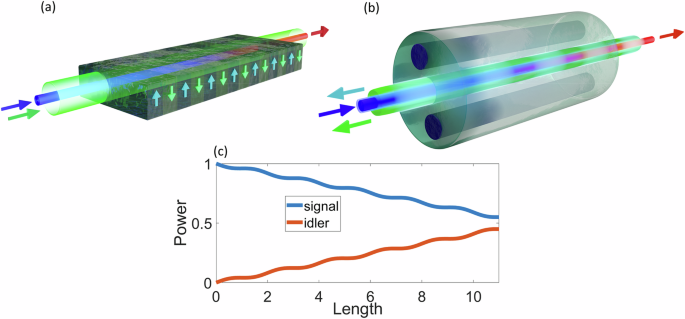
In the case of standard QPM (a), spatial modulation of susceptibility within the optical medium is permanent. This modulation facilitates efficient conversion between input light (signal, indicated by a blue beam) and output light (idler, indicated by a red beam), which co-propagate from left to right and have different wavelengths. In the case of optically programmable QPM (b), the input light (signal wave) is coupled to an unmodified optical fiber that maintains uniformity along its length. Two pump waves involved in the nonlinear process counter-propagate relative to the signal and idler waves. Modulation of one of the pump waves (green beam) enables a process efficiency akin to standard QPM, facilitating the coherent buildup of the output light (signal wave) as illustrated in (c).
Assuming undepleted pumps, where the fast (or slow) pump is time-modulated by a sinusoidal wave with angular frequency \({\omega }_{m}\), we describe the evolution of the signal and idler wavepackets using coupled wave equations (CWE), akin to those seen in a two-level system32. The CWEs are: (for four-field model see Supplementary note 1):
$$\frac{\partial {A}_{s}}{\partial z}=i\gamma {A}_{i}{A}_{p}^{\, f}{{A}_{p}^{s}}^{*}\cos \left({\kappa }_{m}z+{\omega }_{m}t\right)\exp \left(i\Delta {kz}\right)$$
(1)
$$\frac{\partial {A}_{i}}{\partial z}=i\gamma {A}_{s}{A}_{p}^{s}{{A}_{p}^{\, f}}^{*}\cos \left({\kappa }_{m}z+{\omega }_{m}t\right)\exp \left(-i\Delta {kz}\right)$$
(2)
Here \({A}_{p}^{s},{A}_{p}^{\, f},{A}_{i},{A}_{s}\) represent the slowly varying complex envelopes of the pump waves polarized to the slow and fast axes, idler, and signal waves, respectively. Here \(t\) denotes time, and \({\kappa }_{m}=\frac{{\omega }_{m}}{c}n\) is the effective wavenumber of the modulation, where \(c\) is the speed of light, and \(n\) represents the average effective index along the two axes. The Kerr nonlinear coefficient is given by \(\gamma=\frac{3{\chi }^{(3)}\omega }{8{nc}{A}_{{eff}}}\) and is expressed in units of \({W}^{-1}{{km}}^{-1}\), where \({\chi }^{(3)}\) is the third-order susceptibility of the fiber, \(\omega\) is the optical angular frequency, and \({A}_{{eff}}\) is the effective mode area. Since \(n,{\chi }^{(3)},\omega\), and \({A}_{{eff}}\) are sufficiently close in value for all the optical fields considered, we approximate \(\gamma\) as being equal for all fields52. The wavenumber mismatch term is \(\Delta k={k}_{p}^{f}-{k}_{p}^{s}+{k}_{i}-{k}_{s}\), where \({k}_{p}^{\, f},{k}_{p}^{s},{k}_{s},{k}_{i}\) are the wavenumbers of the two pumps, signal, and idler, respectively (see in Fig. 2(a) the illustration of the dispersion relation of the fiber).
Fig. 2: Phase-matching principle and experimental setup for optically programmable QPM.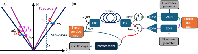
Panel (a) illustrates the dispersion relation between temporal frequency and axial wavenumber for light guided in the slow (dark blue) and fast (purple) axes of a polarization-maintaining (PM) fiber. The signal (represented by full blue circular markers) and the idler (represented by empty circular red marker) propagate forward along the slow and fast axes, respectively, while the slow and fast pump waves (represented by full green and violet circular markers, respectively) propagate backwards. The blue arrows represent the momentum difference between the two pumps, which results in a corresponding momentum mismatch \(\Delta {{{\rm{k}}}}\) between the signal and the idler. The fast pump is modulated to create the optically programmable QPM that will align with the momentum mismatch. Panel (b) provides a schematic illustration of the experimental setup. AOM acousto-optic modulator, EOM electro-optic amplitude modulator, EDFA erbium-doped fiber amplifier, PBS polarization beam splitter.
In the standard case, where there is no pump modulation, i.e., \({\omega }_{m}=0\) and \({\kappa }_{m}=0\), energy conservation dictates the condition \(\Omega={\omega }_{i}-{\omega }_{s}\), where \({\omega }_{i}\) and \({\omega }_{s}\) denote the angular frequencies of the idler and signal waves. In this case, efficient conversion between the signal and idler waves occurs when their wavenumber mismatch is (approximately) \(\Delta k(\Omega,\Delta \omega )\approx \frac{1}{c}\left(2\Omega n-\Delta n\Delta \omega \right)\) where \(\Delta n\) is the birefringence between the two principal axes, and \(\Delta \omega\) is the offset between the signal optical frequency \({\omega }_{s}\) and the pump frequency \({\omega }_{p}^{s}\) (see supplementary note 1). We refer to this as the natural wavenumber mismatch. The corresponding angular frequency difference between the pump and signal is \(\Delta \omega=2\Omega \frac{n}{\Delta n}\).
When pump temporal modulation is applied with an angular frequency \({\omega }_{m}\), Eqs. 1 and 2 resemble the standard QPM equations, where \({\kappa }_{m}\) serves as the wavenumber of the spatial modulation. The temporal term in the sinusoidal wave induces QPM in energy, altering the frequency difference between the idler and signal waves, \({\omega }_{i}-{\omega }_{s}=\Omega \pm {\omega }_{m}\). This frequency shift introduces an additional term to the phase matching condition53, \(\Delta {k}_{t}=\frac{{\omega }_{m}}{c}n\), so the overall spatiotemporal term becomes:
$$\Delta {k}_{{st}}=\Delta {k}_{t}+{\kappa }_{m}=2\frac{{\omega }_{m}}{c}n$$
(3)
(see supplementary note 1). The QPM is satisfied when \(\Delta {k}_{{st}}=\left|\Delta k\right|\). Consequently, the pump-signal frequency difference with maximal coupling is:
$$\Delta {\omega }_{{st}}(\Omega,{\omega }_{m})=\left(2\Omega \pm 2{\omega }_{m}\right)\frac{n}{\Delta n}$$
(4)
where the sign depends on the Fourier terms in \(\sin \left({\kappa }_{m}z+{\omega }_{m}t\right)\). This is a manifestation of spatiotemporal QPM47, where the pump temporal modulation governs both the momentum mismatch \(\Delta {k}_{{st}}\) and the energy mismatch \(\Delta {\omega }_{{st}}\). We note that the ratio \(\frac{n}{\Delta n}\) is quite large (~4300 in our experiment), hence the frequency conversion can be achieved over very broad spectral range by relatively small change in the pump modulation frequency \({\omega }_{m}\).
The interaction we consider includes two pump waves, but the wavelength of efficient coupling can be controlled by temporally modulating only one of the pumps with an angular frequency \({\omega }_{m}\). Furthermore, by applying an additional envelope function \(a(t)\) to the sinusoidal wave, nonuniform QPM can be created along the fiber. This enables to control the spectrum of the coupling efficiency, which can be represented as the Fourier transform \(A(2\delta \frac{\Delta n}{n})\) of the envelope function \(a(t)\), where \(\delta\) is the frequency offset from the exact phase matching condition33 (see Supplementary note 2).
The solution to the CWEs is the same as that of a two-level system28,32. Assuming initially zero idler power at the fiber’s entrance, and completely satisfying the QPM condition, \({\kappa }_{m}=\left|\varDelta k\right|,\) the conversion efficiency to the idler at the fiber’s end (\(z=L\)) is given by:
$$\eta=\frac{{P}_{i}\left(L\right)}{{P}_{s}\left(0\right)}={\sin }^{2}\left(\sqrt{\frac{{\gamma }^{2}{P}_{p}^{\, s}{P}_{p}^{\, f}}{4}}L\right)$$
(5)
Here, \({P}_{s}\),\({P}_{i}\), \({P}_{p}^{\, s}\), and \({P}_{p}^{f}\) represent the signal, idler, slow pump, and fast pump powers, respectively. Note that the factor \(1/4\) in the sinusoidal argument accounts for the presence of two QPM orders (negative and positive), but only one is effective for each wavelength.
In the regime of relatively low efficiency, where \(\sqrt{\frac{{\gamma }^{2}{P}_{p}^{s}{P}_{p}^{\,f}}{4}}L\, \ll \,1\), the sine function can be approximated as a linear function. Under this approximation, the conversion efficiency simplifies to \(\eta \approx \frac{{\gamma }^{2}{P}_{p}^{\, s}{P}_{p}^{\, f}}{4}{L}^{2}\).
Experimental results
The optically programable QPM setup is illustrated in Fig. 2. The pump waves were generated from a fiber laser at 1550 nm, which was split into two branches, and both of them coupled to the exit port of the fiber, \(z=L\). In one branch, the optical wave was upshifted by a fixed intermediate frequency offset of \(\frac{\Omega }{2\pi }=\)200 MHz using an acousto-optic modulator. This served as the non-modulated pump and was coupled to the slow axis of 30 m panda-type PM fiber via a circulator A, and polarization beam splitter (PBS). In the other branch, modulation was applied to the second pump by an electro-optic modulator driven by an arbitrary waveform generator and coupled to the fast axis of the fiber from the same edge via circulator B. The modulator is biased to the minimum power operating point, where the optical field response is linear with respect to the applied voltage. The average power of each of the two pumps was amplified to 80 mW.
A continuous-wave signal wave from a tunable diode laser was also split into two branches. One branch served as a local oscillator (LO), while the other, serving as the signal wave, was coupled to the slow axis of the PM fiber from the entrance port of the fiber, \(z=0\). Owing to the nonlinear interaction, part of the signal wave was converted to the orthogonally polarized idler, which propagated through the fast arm of the PM fiber and was sent using the PBS and circulator B towards a PM coupler, where it was mixed with the LO and detected using a photoreceiver, over acquisition time of \(\Delta \tau\). Prior to detection, both the LO and idler passed through optical bandpass filters to suppress any residual pump leakage (the bandpass filters are not shown in the setup). The Fourier Transform \(\widetilde{V}(\omega )\) of the detected voltage \(v(t)\) was analyzed offline, and the square of Fourier Transform magnitude \({\left|\widetilde{V}\left(\Omega \pm {\omega }_{m}\right)\right|}^{2}\) was proportional to the idler power.
Figure 3 depicts the idler normalized output power as a function of wavelength for various QPM frequencies. In all panels of Fig. 3, the acquisition time was \(\Delta \tau=1\mu s\), and the absolute value of the Fourier Transform of the voltage \(\left|V\left(\omega \right)\right|\) was averaged offline over 256 times. We fine-tuned the pump wavelength in the simulation by tens of picometers to precisely match the experimental conditions and eliminate any wavelength drifting effects. Panel (a) presents the idler power without any QPM, with the maximum coupling near 1538 nm corresponding to a birefringence of \(\Delta n\approx 3.4\times {10}^{-4}\). The dashed line represents numerical calculations (see details in the method section). Panel (b) shows the same for a QPM frequency of \({\omega }_{m}/2\pi=\) 100 MHz, with the maximum coupling near 1532 nm. Panel (c) is analogous to panel (a) but with a QPM of \({\omega }_{m}/2\pi=\) 400 MHz, resulting in maximum coupling near 1562 nm. Here, the wavelength of maximum coupling is above the natural phase-matching wavelength observed in panel (a), as the phase matching is due to the negative order of the QPM. Panel (d) presents the wavelength of maximum coupling as a function of the QPM frequency, with negative frequencies indicating the negative (−1) order of QPM. The red markers present measurements, while the blue line presents theoretical analysis. As shown in the figure, by varying the QPM frequency by less than 800 MHz, phase matching can be achieved over a spectral range of 80 nm, covering the entire C-band and L-band of optical telecom. Additionally, we demonstrate coupling at 1312 nm. In this experiment, as shown in the rightmost inset, we did not vary the signal wavelength (as in the other experiments) but instead swept over the QPM frequency and found maximum coupling near 4.3 GHz. Together, these experiments demonstrate tunability over a spectral range of 298 nm. The deviation from the ideal sinc function is attributed to inhomogeneities in the fiber’s birefringence along its length48.
Fig. 3: Experimental and theoretical demonstration of wavelength-tunable signal-idler coupling via optically programmable QPM.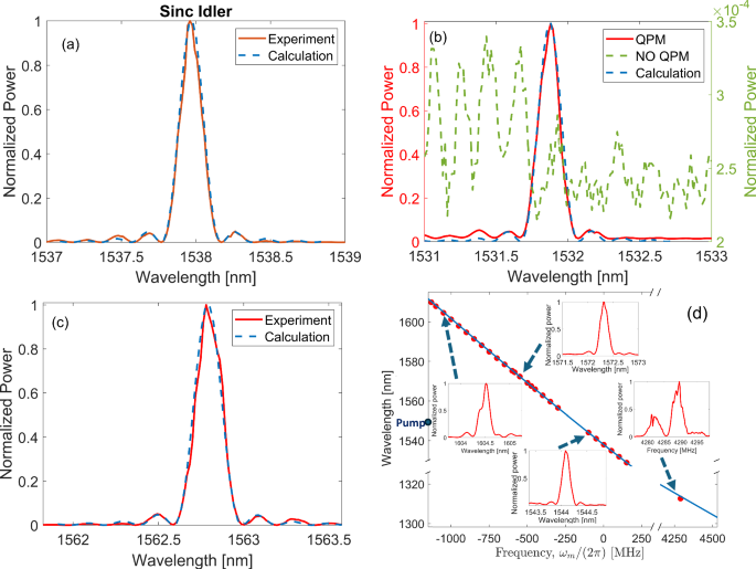
a presents the normalized signal-idler coupling spectrum under natural phase matching conditions, where no QPM is applied. The red line represents experimental data, while the well-matched, dashed blue line depicts numerical calculations. Panel (b) illustrates the same scenario as a but with a QPM frequency of \({\omega }_{m}/2\pi=\) 100 MHz. The green line represents the signal-idler coupling without QPM. A striking difference of more than three orders of magnitude is observed between coupling with and without QPM. c mirrors a and b but with a QPM frequency of \({\omega }_{m}/2\pi=\) 400 MHz. Here, the maximum coupling occurs near 1562.8 nm, corresponding to the negative order of the QPM. d summarizes 27 measurements conducted with different QPM frequencies \({\omega }_{m}/2\pi\) ranging from 50 MHz to 4.3 GHz. The graph demonstrates the tunability of the spectrum over a wide range of 298 nm. The insets show examples of the measurements that contribute to the main graph. The red markers represent the experimental measurements, while the blue line corresponds to the theoretical analysis. According to the theory, the optical frequency is linearly dependent on the QPM frequency (see Eq. 4). The theoretical line has linear dependence on frequency (Eq. 4), but since it is shown here as a function of wavelength, its slope varies.
Figure 4 demonstrates the impact of adding an envelope modulation to the sinusoidal wave, which in turn modulates the pump, with various pulse shapes. The normalized coupling spectrum is depicted when the QPM frequency is \({\omega }_{m}/2\pi\) = 100 MHz. In all panels, the absolute value of the Fourier Transform of the voltage \(\left|V\left(\omega \right)\right|\) was averaged offline over 512 repeating pump pulses. The experimental data in all panels is represented by a solid red line, while the dashed line represents the simulation. We adjusted the pump wavelength in the simulation by tens of picometers to match the experiment and prevent wavelength drifting effects. The pulse duration was 40 ns in all panels, denoted by \(T\). The insets in all panels correspond to the generated arbitrary waveform voltage before amplification. In a, where there is no envelope modulation to the sine wave, the spectrum is simply governed by the length of the PM fiber and takes the shape of the sinc function. The acquisition time for this panel was \(\Delta \tau=1\mu s\). For b–d, the acquisition time was \(\Delta \tau=20{ns}\), synchronized with the arbitrary waveform generator. In panel (b), the sinusoidal wave was modulated by a Gaussian pulse \(a\left(t\right)=\exp \left(-\frac{1}{2}{\left(\frac{t}{T}\right)}^{2}\right)\). As expected, the spectrum resembles the Fourier Transform of the pulse, which is also Gaussian. Panel (c) features a pulse shape characterized by the normalized sinc function \(a\left(t\right)=\sin \left(\frac{\pi t}{T}\right)/\frac{\pi t}{T}\), resulting in a rectangular coupling spectrum. In panel (d), the pulse shape corresponds to the first Hermite-Gauss polynomial, \(a\left(t\right)={{{\rm{t}}}}\times \exp \left(-\frac{1}{2}{\left(\frac{t}{T}\right)}^{2}\right)\), with the resulting spectrum also displaying the dual-lobe Hermite-Gauss characteristics.
Fig. 4: Signal-Idler coupling spectra with various pulse shapes.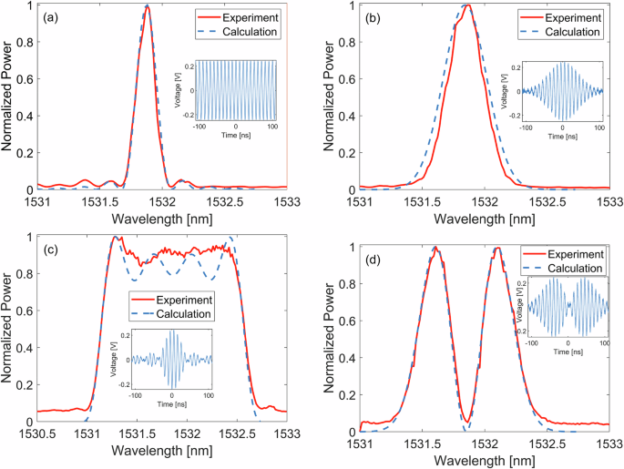
a Normalized spectrum of idler power when the fast pump is modulated by a pure sinusoidal wave of \(\frac{{\omega }_{m}}{2\pi }=\)100 MHz. The spectrum exhibits a sinc shape, corresponding to the Fourier transform of a rectangular function (over a 30 m PM fiber). Experimental data is represented by the solid red line, while numerical calculations are depicted by the dashed blue line. b–d replicate the scenario presented in (a), with the sinusoidal wave modulated by Gaussian, sinc, and the first Hermite-Gauss polynomial, respectively. In each case, the measured spectra represent the Fourier transform of the respective pulse shape: Gaussian for b, rectangular for c, and the first Hermite-Gauss polynomial for d. Inset graphs in each panel display the temporal voltage waveform used to modulate the fast pump light, illustrating the pulse shapes applied.
Figure 5 illustrates the conversion efficiency to the idler wave as a function of the pump power. In panel (a), the PM fiber mirrors the parameters outlined in Figs. 4 and 3, spanning a length of 30 meters, with the signal power set at 3 mW and the fast pump power maintained at 670 mW. The slow pump power is monotonically varied from 30 to 300 mW. Experimental data, denoted by the solid red line, closely aligns with theoretical calculations represented by the dashed blue line. Notably, the data indicate a maximum efficiency of \(7.5\times {10}^{-3}\) %. In panel (b), a shift is observed as the PM fiber transitions to a 440 m PM panda-type fiber. Here, the fast pump power is held constant at 1 W, while the fast pump power undergoes adjustments from 180 mW to 1 W. The maximum efficiency attained in this configuration reaches 5.4%. The pump light source is broadened to 300 MHz through phase modulation via pseudo-random binary sequence, in order to mitigate the influence of spontaneous Brillouin scattering, that may limit the process efficiency. Theoretical underpinnings, corroborated by experimental findings, delineate a clear relationship between efficiency, fiber length, and pump power. Specifically, in relatively low efficiency \(\eta \ll 1\), the efficiency is shown to scale quadratically with the fiber length and linearly with each of the pump powers, aligning with established theoretical frameworks and empirical observations. The partial discrepancy between the measurement and the theoretical model in panel (b) is due to a lack of uniformity in the birefringence along the fiber48 which leads to an effective interaction length that is shorter than the actual physical length of the fiber. Data analysis indicates that the effective length in this case is 356 m.
Fig. 5: Efficiency dependence on slow pump power for short and long fibers.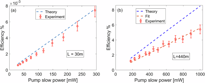
a illustrates the efficiency of the process as a function of slow pump power, with the fast pump set at 670 mW and the fiber length at 30 m. Experimental data is depicted by the red markers, which include vertical error bars representing the standard deviation, while theoretical analysis is represented by the dashed blue line. b mirrors a but with the fast pump fixed at 1 W. Additionally, the fiber length is extended to 440 m. The dashed red line is a fit to the experimental data, indicating an effective length of 356 m.
The measured efficiency, even at the high pump power, justifies our assumption of the undepleted pump approximation. However, with higher conversion efficiency, this analysis can be further extended to the depleted pump regime32.