Mathematical operations for physical dimensions and units
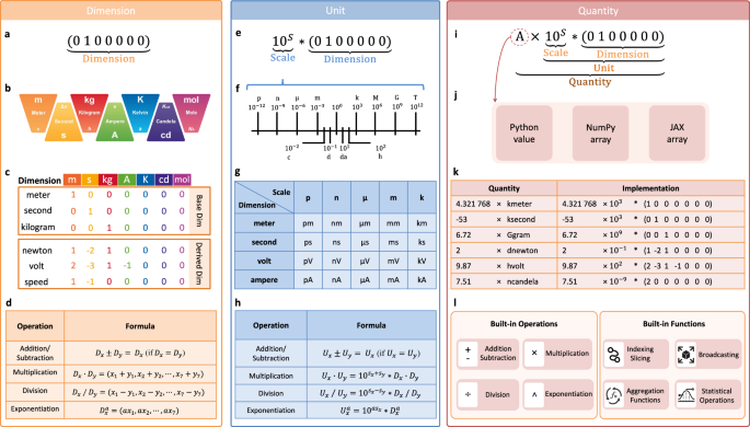
In the dimensional analysis of physical units, fundamental operations include addition, subtraction, multiplication, division, and exponentiation (see Fig. 1d and Table 1 for saiunit.Dimension, and Fig. 1h and Table 1 for saiunit.Unit). These operations are governed by rigorous mathematical rules by the SI standard14, ensuring both correctness and consistency in the treatment of physical dimensions. Particularly, addition and subtraction are permitted only when the dimensional types are compatible. Physical units need to adjust compatible scale factors when performing addition and subtraction. Multiplication and division, however, are unconstrained by such compatibility requirements, while exponentiation is permitted not only for scalar exponents. Further details can be found in Table 1.
Table 1 Operational rules for physical dimensions and unitsUnit-compatible gradient computation with JAX AD
Unit-aware computations in SAIUnit support two types of gradient computations. The first type employs the original JAX AD, wherein gradients preserve the original data’s units because JAX AD treats quantities with physical units as PyTrees. Physical quantities in SAIUnit seamlessly support both forward and reverse AD of JAX. This includes operations such as scalar loss gradients using jax.grad, forward-mode Jacobian computations with jax.jacfwd, reverse-mode Jacobian computations with jax.jacrev, and Hessian matrix computations using jax.hessian. During forward computations, the unit system ensures consistency among data units. However, during the AD pass, unit checking is disabled, and units are not enforced among gradients. Whether using forward-mode or reverse-mode gradient passes, the computed gradients retain the same units as the original data. This feature — treating units as static data that do not propagate through gradient computations — is very useful to be directly compatible with traditional AD optimizers.
Unit-aware gradient computation with saiunit.autograd
The second gradient computation within SAIUnit is provided in saiunit.autograd module, which ensures all derivative operations respect the dimensions and units of the involved quantities and maintains physical interpretability of derivatives. saiunit.autograd establishes a formal mathematical framework for unit-aware AD, which encompasses scalar-loss gradients, Jacobians via forward-mode AD, Jacobians via reverse-mode AD, and Hessians. By formalizing AD operations with unit-aware rules, we ensure that derivatives not only are mathematically correct but also physically meaningful. For a concrete example of unit-aware automatic differentiation, please refer to Supplementary Note H.
Unit-aware scalar-loss gradient: saiunit.autograd.grad
For a scalar-valued differentiable function \(f:{{\mathbb{R}}}^{n}\to {\mathbb{R}}\), where each input \({x}_{i}\in {\mathbb{R}}\) is associated with a physical quantity qi having dimension [qi]. The output f(x) has its own dimension [f]. The gradient ∇ f(x) is a vector in \({{\mathbb{R}}}^{n}\) consisting of the first partial derivatives of f with respect to each component of x:
$$\nabla f({{{\bf{x}}}})={\left[\frac{\partial f}{\partial {x}_{1}}({{{\bf{x}}}}),\frac{\partial f}{\partial {x}_{2}}({{{\bf{x}}}}),\ldots,\frac{\partial f}{\partial {x}_{n}}({{{\bf{x}}}})\right]}^{T},$$
(1)
where each component \(\frac{\partial f}{\partial {x}_{i}}\) has dimensions \(\left[\frac{\partial f}{\partial {x}_{i}}\right]=\frac{[f]}{[{x}_{i}]}\). For example, if f has units of energy [E] (e.g., joules), and xi has units of length [L] (e.g., meters), then \(\left[\frac{\partial f}{\partial {x}_{i}}\right]=\frac{[E]}{[L]}\), which corresponds to force units [F] = [E]/[L].
Unit-aware jacobian: saiunit.autograd.jacfwd and saiunit.autograd.jacrev
For a vector-valued function \({{{\bf{f}}}}:{{\mathbb{R}}}^{n}\to {{\mathbb{R}}}^{m}\), each component \({f}_{j}:{{\mathbb{R}}}^{n}\to {\mathbb{R}}\) has its own dimension [fj]. The Jacobian matrix Jf(x) computed using reverse-mode (saiunit.autograd.jacrev) or forward-mode AD (saiunit.autograd.jacfwd) is an m × n matrix where each entry (i, j) is the partial derivative of the i-th component of f concerning the j-th component of x.
$${J}_{{{{\bf{f}}}}}({{{\bf{x}}}})=\left[\begin{array}{cccc}\frac{\partial {f}_{1}}{\partial {x}_{1}}({{{\bf{x}}}})&\frac{\partial {f}_{1}}{\partial {x}_{2}}({{{\bf{x}}}})&\ldots &\frac{\partial {f}_{1}}{\partial {x}_{n}}({{{\bf{x}}}})\\ \frac{\partial {f}_{2}}{\partial {x}_{1}}({{{\bf{x}}}})&\frac{\partial {f}_{2}}{\partial {x}_{2}}({{{\bf{x}}}})&\ldots &\frac{\partial {f}_{2}}{\partial {x}_{n}}({{{\bf{x}}}})\\ \vdots &\vdots &\ddots &\vdots \\ \frac{\partial {f}_{m}}{\partial {x}_{1}}({{{\bf{x}}}})&\frac{\partial {f}_{m}}{\partial {x}_{2}}({{{\bf{x}}}})&\ldots &\frac{\partial {f}_{m}}{\partial {x}_{n}}({{{\bf{x}}}})\end{array}\right],$$
(2)
where each entry \(\frac{\partial {f}_{i}}{\partial {x}_{j}}\) has dimensions \(\frac{[{f}_{i}]}{[{x}_{j}]}\).
Unit-aware Hessian: saiunit.autograd.hessian
For a scalar-valued twice-differentiable function \(f:{{\mathbb{R}}}^{n}\to {\mathbb{R}}\), the Hessian matrix Hf(x) at x is an n × n symmetric matrix consisting of all second-order partial derivatives of f:
$${H}_{f}({{{\bf{x}}}})=\left[\begin{array}{cccc}\frac{{\partial }^{2}f}{\partial {x}_{1}^{2}}({{{\bf{x}}}})&\frac{{\partial }^{2}f}{\partial {x}_{1}\partial {x}_{2}}({{{\bf{x}}}})&\ldots &\frac{{\partial }^{2}f}{\partial {x}_{1}\partial {x}_{n}}({{{\bf{x}}}})\\ \frac{{\partial }^{2}f}{\partial {x}_{2}\partial {x}_{1}}({{{\bf{x}}}})&\frac{{\partial }^{2}f}{\partial {x}_{2}^{2}}({{{\bf{x}}}})&\ldots &\frac{{\partial }^{2}f}{\partial {x}_{2}\partial {x}_{n}}({{{\bf{x}}}})\\ \vdots &\vdots &\ddots &\vdots \\ \frac{{\partial }^{2}f}{\partial {x}_{n}\partial {x}_{1}}({{{\bf{x}}}})&\frac{{\partial }^{2}f}{\partial {x}_{n}\partial {x}_{2}}({{{\bf{x}}}})&\ldots &\frac{{\partial }^{2}f}{\partial {x}_{n}^{2}}({{{\bf{x}}}})\end{array}\right],$$
(3)
where each second-order partial derivative \(\frac{{\partial }^{2}f}{\partial {x}_{i}\partial {x}_{j}}\) has dimensions \(\frac{[f]}{[{x}_{i}][{x}_{j}]}\).
Chain rule with units
When composing functions, the chain rule must respect units. For functions \(f:{{\mathbb{R}}}^{n}\to {{\mathbb{R}}}^{m}\) and \(g:{{\mathbb{R}}}^{m}\to {{\mathbb{R}}}^{p}\):
$$\frac{\partial {(g\cdot f)}_{k}}{\partial {x}_{i}}={\sum}_{j=1}^{m}\frac{\partial {g}_{k}}{\partial {f}_{j}}\frac{\partial {f}_{j}}{\partial {x}_{i}}.$$
(4)
The physical dimensions should follow the rule of:
$$\left[\frac{\partial {(g\cdot f)}_{k}}{\partial {x}_{i}}\right]=\frac{[{g}_{k}]}{[{x}_{i}]}={\sum}_{j=1}^{m}\left(\frac{[{g}_{k}]}{[{f}_{j}]}\cdot \frac{[{f}_{j}]}{[{x}_{i}]}\right)$$
(5)
where each term in the sum maintains \(\frac{[{g}_{k}]}{[{f}_{j}]}\cdot \frac{[{f}_{j}]}{[{x}_{i}]}=\frac{[{g}_{k}]}{[{x}_{i}]}\).
Linearity of differentiation with units
For any scalar constants a, b with appropriate dimensions and functions \(f,g:{{\mathbb{R}}}^{n}\to {\mathbb{R}}\):
$$\frac{\partial }{\partial {x}_{i}}(af+bg)=a\frac{\partial f}{\partial {x}_{i}}+b\frac{\partial g}{\partial {x}_{i}}.$$
(6)
The physical dimensions should follow the rule of:
$$\left[\frac{\partial }{\partial {x}_{i}}(af+bg)\right]=\frac{[af+bg]}{[{x}_{i}]}=\frac{[a][f]+[b][g]}{[{x}_{i}]},$$
(7)
where each term on the right-hand side has:
$$\left[a\frac{\partial f}{\partial {x}_{i}}\right]=[a]\cdot \frac{[f]}{[{x}_{i}]},\quad \left[b\frac{\partial g}{\partial {x}_{i}}\right]=[b]\cdot \frac{[g]}{[{x}_{i}]}$$
(8)
For dimensional consistency, [a][f] = [b][g].
Integrating physical units into scientific computing libraries
There are two primary methods for integrating SAIUnit’s unit-aware system into scientific computing libraries across various domains.
Method 1: deep integration of SAIUnit into scientific computing libraries
The first method involves deeply integrating SAIUnit into scientific computing libraries, as demonstrated in Seamless integration of unit-aware computations across disciplines with libraries such as Diffrax, BrainPy, and PINNx. The core steps of this integration include:
-
Representing arrays with SAIUnit’s quantity: Data is represented using saiunit.Quantity instead of jax.Array, thereby assigning explicit physical dimensions to the data. This ensures that the data possesses consistent and traceable unit information before numerical computations.
-
Utilizing SAIUnit’s unit-aware mathematical functions: During computations, mathematical functions from the saiunit.math module are employed instead of those from jax.numpy. This approach maintains unit awareness and facilitates unit conversions throughout the numerical calculation process.
Since SAIUnit is designed as a comprehensive, unit-aware, NumPy-like computational library, these two steps typically suffice to seamlessly integrate unit-aware computations into scientific computing libraries. However, specific implementations may exhibit subtle differences across different scientific computing libraries (see following sections).
Method 2: Encapsulating unit support for predefined scientific computing functions
A substantial number of existing scientific computing functions are designed based on dimensionless data. The second method applies to these dimensionless functions without modifying existing frameworks or underlying implementations. The core idea is:
-
Dimensionless processing before function calls: Before invoking scientific computing functions, input data undergoes dimensionless processing to ensure that the functions internally handle only unitless numerical operations. For example, using b = a.to_decimal(UNIT) method can normalize the quantity a into the dimensionless data b according to the given physical unit UNIT.
-
Restoring physical units after computation: Once the computation is complete and results are returned, we can restore the appropriate physical units to the solutions.
Specifically, SAIUnit provides the assign_units function, which facilitates the automatic assignment and restoration of physical units at the input and output stages of functions. This method is, in principle, applicable to any Python-based scientific computing library, preserving the physical semantics and interpretability at the input and output levels without altering their existing structures. Supplementary Note C shows an example of integrating physical units into SciPy’s optimization functionalities using assign_units function.
Integrating physical units into numerical integration
We have integrated SAIUnit into the numerical solver library Diffrax22, enabling physical unit checks and constraints during the integration process. We integrated SAIUnit into Diffrax by considering not only defining physically meaningful variables as shown in Supplementary Note I, but also providing robust dimensional consistency verification throughout the computation process. When constructing differential equations, the unit-aware Diffrax rigorously enforces dimensional compatibility between the right-hand side parameters and variables and their left-hand side counterparts. During numerical integration, the solver performs comprehensive unit validation at each step, ensuring that all intermediate variables and parameters maintain dimensional consistency according to standardized measurement units. This verification process also generates immediate diagnostic feedback through error messages if any dimensional inconsistencies are detected, allowing users to identify and rectify potential physical modeling errors early in their calculations.
Integrating physical units into brain modeling
SAIUnit has been deeply integrated into the brain dynamics programming ecosystem BrainPy18,19. This integration ensures that BrainPy users can now seamlessly incorporate physical units into their brain modeling workflows, including not only biophysical single neuron models (see Supplementary Note B), but also circuit networks (see Supplementary Note E and F). Particularly, we integrated physical units into BrainPy to enable precise expression and tracking of key biophysical quantities during the modeling process, including basic physical quantities such as membrane potential (mV), ion concentration (mol/L), and synaptic conductance (nS), as well as multi-scale dynamical features ranging from millisecond-scale action potentials to hour-long neural activity, and from micron-scale synaptic structures to centimeter-scale brain regions. Given that neuroscience experimental data inherently carries physical units, we have integrated SAIUnit into the experimental data fitting process of BrainPy, enabling direct comparison of simulation results with experimental data.
Integrating physical units into PINNs
We have integrated SAIUnit with PINNx to create unit-aware PINNs. This integration addresses key limitations of existing PINN methods and frameworks, which often lack explicit physical meanings. One significant challenge with current PINN libraries, such as DeepXDE32, is that they require users to manually track the order and meaning of variables. For instance, in these frameworks, variables[0] might represent the amplitude, variables[1] the frequency, and so on, without any intrinsic connection between the variable order and its physical meaning. In contrast, PINNx allows users to assign explicit, meaningful names to variables (e.g., variables[“amplitude”] and variables[“frequency”]), removing the need to manage the order of variables manually.
Another limitation of existing PINN libraries is their reliance on users to manage complex Jacobian and Hessian relationships among variables. In PINNx, we simplify this by tracking intuitive gradient relationships through simple dictionary indexing. For example, users can access the Hessian matrix ∂2y/∂x2 using hessian[“y”][“x”][“x”] and the Jacobian matrix ∂y/∂t with jacobian[“y”][“t”].
Additionally, many existing PINN frameworks lack native support for physical units, which is essential for ensuring dimensional consistency in physical equations. For instance, in the Burgers equation, the left-hand side \(\frac{\partial u}{\partial t}+u\frac{\partial u}{\partial x}\) and the right-hand side \(\nu \frac{{\partial }^{2}u}{\partial {x}^{2}}\) must have the same physical units, meter/second2. To address this, PINNx leverages unit-aware automatic differentiation from saiunit.autograd, enabling the computation of first-, second-, or higher-order derivatives while preserving unit information. This ensures that physical dimensions are correctly maintained throughout the derivation process.
Supplementary Note I demonstrates how to implement a unit-aware PINN to solve one-dimensional Burgers equation using SAIUnit.
Integrating physical units into JAX, M.D. and catalax
We have also integrated physical units into JAX, M.D.21 and Catalax23 using both deep integration and encapsulation methods. We incorporated physical units such as electric voltage, angstrom, interatomic force, and atomic mass units to quantify force, temperature, pressure, and stress within molecular dynamics simulations. Most energy and displacement functions were computed using unit-aware mathematical functions from SAIUnit, ensuring automatic unit conversion and validation when defining molecular quantities. However, for energy potentials computed by neural networks in JAX, M.D., we used assign_units to convert quantities with units into dimensionless data, allowing for their processing by neural networks. Afterward, the energy units were restored to ensure an accurate representation of the simulation results. In Catalax, we enabled unit-aware biological systems modeling by integrating physical units into its differential equation definitions. We employed our unit-aware Diffrax for numerical integration and utilized assign_units for Markov Chain Monte Carlo (MCMC) sampling when fitting experimental data distributions, as the underlying MCMC interface is inherently dimensionless.
Computing calcium currents using Goldman-Hodgkin-Katz equation
The low-threshold voltage-activated T-type calcium current in the Cerebellum Purkinje cell model was modeled in Haroon et al.30. This model incorporates two activation gates (m) and one inactivation gate (h), capturing the channel’s gating dynamics. The current density is calculated using the Goldman-Hodgkin-Katz (GHK) equation28, which accounts for the electrochemical gradients of calcium ions across the neuronal membrane. The kinetic equations governing the T-type calcium current are summarized below:
$${I}_{{{{{\rm{Ca}}}}}^{2+}}=\overline{{P}_{{{{{\rm{Ca}}}}}^{2+}}}\times {m}^{2}\times h\times {g}_{{{{\rm{GHK}}}}}$$
(9)
$$\frac{{{{\rm{d}}}}m}{{{{\rm{d}}}}t}=\frac{{m}_{\infty }-m}{{\tau }_{m}}$$
(10)
$${\tau }_{m}=\left\{\begin{array}{ll}1\hfill\quad &\,{{\rm{if}}}\,V \, \leqslant -90\,{{{\rm{mV}}}},\\ 1+\frac{1}{\exp \left(\frac{V+40}{9}\right)+\exp \left(-\frac{V+102}{18}\right)}\quad &\,{{\rm{otherwise}}}\,,\end{array}\right.$$
(11)
$${m}_{\infty }=\frac{1}{1+\exp \left(-\frac{V+52}{5}\right)}$$
(12)
$$\frac{{{{\rm{d}}}}h}{{{{\rm{d}}}}t}=\frac{{h}_{\infty }-h}{{\tau }_{h}}$$
(13)
$${h}_{\infty }=\frac{1}{1+\exp \left(\frac{V+72}{7}\right)}$$
(14)
$${\tau }_{h}=15+\frac{1}{\exp \left(\frac{V+32}{7}\right)}.$$
(15)
Where \(\overline{{P}_{{{{{\rm{Ca}}}}}^{2+}}}\) represents the maximal permeability of the channel to calcium ions which has the units of cm ⋅ second−1, and gGHK is the Goldman-Hodgkin-Katz conductance, defined as:
$${g}_{{{{\rm{GHK}}}}}={z}^{2}\frac{{V}_{m}{F}^{2}}{RT}\frac{{[{{{\rm{C}}}}]}_{i}-{[{{{\rm{C}}}}]}_{o}\exp \left(-z{V}_{m}F/RT\right)}{1-\exp \left(-z{V}_{m}F/RT\right)},$$
(16)
in which z = 2 is the valence of the calcium ion, Vm is the membrane potential which is measured in mV, F = 96485.3321 s ⋅ A ⋅ mol−1 is the Faraday constant, R = 8.3144598 J ⋅ mol−1 ⋅ K−1 is the universal gas constant, T = 295.15 K is the temperature, [C]i and [C]o = 2.0 mM are the intracellular and extracellular calcium ion concentrations, respectively.
The activation variable m and the inactivation variable h evolve over time according to their respective steady-state values (m∞ and h∞) and time constants (τm and τh). These dynamics ensure that the T-type calcium current responds appropriately to changes in membrane potential.
In the NEURON simulator, the absence of intrinsic physical units necessitates most dimensional scaling to be performed manually. Initially, the membrane voltage Vm is represented as a dimensionless quantity scaled by the unit mV. This voltage is then converted to volts (V) as shown in Line 04 of Fig. 5b, resulting in the dimensionless parameter \(\zeta=\frac{z{V}_{m}F}{RT}\) (Line 05 in Fig. 5b). The computed conductance gGHK initially has units of C/m3. However, since the permeability \(\overline{{P}_{{{{{\rm{Ca}}}}}^{2+}}}\) is measured in centimeters (cm) and the calcium current \({I}_{{{{{\rm{Ca}}}}}^{2+}}\) is calculated based on a membrane area with units of square centimeters (cm2), the NEURON simulator converts gGHK from C/m3 to C/cm3 (Lines 08–10 in Fig. 5b). Finally, to ensure consistency with other ion channel currents, the simulator transforms the calcium current \({I}_{{{{{\rm{Ca}}}}}^{2+}}\) from amperes per cubic centimeter (A/cm3) to milliamperes per cubic centimeter (mA/cm3) (Line 16 in Fig. 5b). For complete details of the NEURON code, please refer to Supplementary Note J.
In contrast, the BrainCell simulator, enhanced by the unit-aware computations of SAIUnit, eliminates the need for researchers to manually manage dimensional scaling. All units are automatically aligned within a unified unit system, allowing physical quantities with differing metric scales to be seamlessly computed together. This automatic alignment ensures consistency and accuracy across simulations, reducing the potential for unit-related errors. Consequently, researchers can focus more on modeling and analysis without worrying about the complexities of unit conversions and dimensional inconsistencies. For a detailed BrainCell code, please refer to Supplementary Note K. For a comparison between NEURON and BrainCell, please refer to Fig. 5b, c.
Environment settings
All evaluations and benchmarks in this study were conducted in a Python 3.12 environment on a system running the Ubuntu 24.04 LTS edition with CPU, GPU, and TPU devices. The CPU experiments ran on an Intel Xeon W-2255, a 10-core/20-thread Cascade Lake processor with a 3.7 GHz base clock and 4.5 GHz turbo boost. The CPU features 24.75 MB of L3 cache and supports up to 512 GB of six-channel DDR4-2933 ECC memory. The GPU experiments used an NVIDIA RTX A6000, a professional Ampere GPU with 10,752 CUDA cores, 336 tensor cores, and 48 GB of GDDR6 memory. The card delivers 1 TB/s memory bandwidth, draws 300W power, and connects via PCIe 4.0 × 16, making it ideal for parallel computing and AI workloads. The TPU experiments leveraged the Kaggle-free TPU v3-8 cloud instance. Specifically, the v3-8 instance gives 8 TPU v3 cores, each providing 128 GB/s of bandwidth to high-performance HBM memory.
The following software versions were used or compared during the study: JAX (v0.4.36)11, BrainPy (v2.6.0)18,19, BrainCell (v0.0.1)20, pinnx (v0.0.1)17, Diffrax (v0.6.1)33, SAIUnit (v0.0.8)34, brainstate (v0.1.0)35, and brainscale36.