Introducing the kernel descent optimizer for variational quantum algorithms

In this section, we present a detailed experimental comparison of kernel descent with $L=1$ versus gradient descent, as well as kernel descent with $L=2$ versus quantum analytic descent. As explained in Sect. 2.5, these pairings are chosen because of their roughly equivalent computational efforts in terms of circuit evaluations per iteration. The experiments are conducted in two main parts. The first part, described in Sects. 3.1, 3.2, and 3.3, is concerned with randomized circuits and observables. This approach allows us to consider a large, statistically significant number of such circuits and observables. The first part is structured as follows:

The algorithms will be compared with respect to the quality of the local approximations (Sect. 3.2) and their performance in terms of their ability to minimize the objective function (Sect. 3.3). Before that, we describe the experimental setup in Sect. 3.1.

In the second part, which is comprised of Sect. 3.4, we deal with a problem from the literature on VQAs.

Setup for experiments with randomized circuits and observables

Here we describe the setup for our experiments in Sects. 3.2 and 3.3. In these experiments we neither take measurement shot noise nor quantum hardware noise into account. That is, all compared algorithms are provided with exact values of the objective function f computed via statevector simulation.

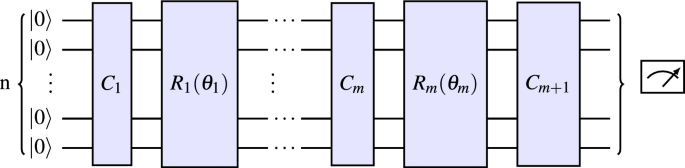
In order to ensure independence of our results from any particular choice of circuit or configuration, we repeatedly sample circuits, observables, and points in parameter space randomly in all our experiments. We proceed similarly to the experimental setup in15: Points in parameter space are randomly sampled from the uniform distribution on $[-\pi , \pi )^m$. With the notation from Sect. 2.1, the observable $\mathcal {M}$ is an n-qubit Pauli randomly sampled from the uniform distribution on $\{I,X,Y,Z\}^{\otimes n}\setminus \{I^{\otimes n}\}$. The generators $G_1, \dots , G_m$ of the parametrized gates $R_1, \dots , R_m$ are sampled (independently) from the uniform distribution on $\{I,X,Y,Z\}^{\otimes n}\setminus \{I^{\otimes n}\}$, and the n-qubit unitaries $C_1, \dots , C_{m+1}$ are randomly sampled (independently) via the same procedure by which the individual layers in the well-known quantum volume test27 are sampled. For a visual representation of the entire circuit we refer to Fig. 1, the specific choice of the unitaries $C_j$ is explained and visualized in Fig. 2.

Figure 2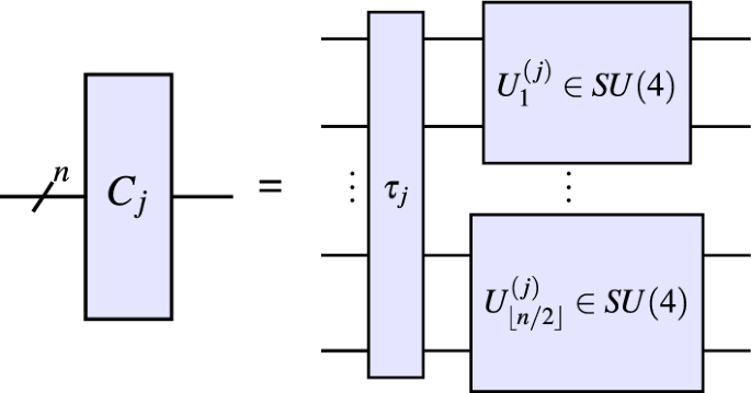

This figure shows the specific choice of unitaries $C_j$ featuring in the experiments in Sects. 3.2 and 3.3: First, a permutation $\tau _j\in S_n$ is sampled uniformly at random. Subsequently, unitaries $U^{(j)}_1,\dots , U^{(j)}_{\left\lfloor {n/2}\right\rfloor }$ are sampled independently from the Haar measure on SU(4). These are then applied to the qubit pairs $(\tau _j (1),\tau _j (2)),\dots ,(\tau _j (2{\left\lfloor {n/2}\right\rfloor }-1),\tau _j (2{\left\lfloor {n/2}\right\rfloor }))$ respectively. Note that this is precisely how the individual layers in the quantum volume test27 are sampled.

Quality of the local approximations

Let $p\in \mathbb {R}^m$ be a point in parameter space, let $g:\mathbb {R}^m\rightarrow \mathbb {R}$ be a local approximation of f about p. In this subsection we will provide comparisons of the two algorithm pairs kernel descent with $L=1$ versus gradient descent and kernel descent with $L=2$ versus quantum analytic descent with respect to three notions of error at a point $\theta \in \mathbb {R}^m$ that is “sufficiently close” to the development point p:

The value approximation error

$$|f(\theta )-g(\theta )|,$$

which is the absolute value of the difference between the value of the true function and that of the local approximation.
The gradient approximation error in Euclidean norm

$$\Vert \nabla {f}(\theta )-\nabla {g}(\theta )\Vert ,$$

which is the Euclidean norm of the difference between the gradient of the true function and that of the local approximation (recall that this is relevant, since all compared algorithms—either explicitly or implicitly—apply gradient descent to the respective local approximations in an inner minimization loop).
The gradient approximation error in cosine distance. That is, the cosine distance between the gradient of the true function and that of the local approximation

$$1-\frac{\nabla {f}(\theta )\bullet \nabla {g}(\theta )}{\Vert \nabla {f}(\theta )\Vert \Vert \nabla {g}(\theta )\Vert },$$

where $\bullet$ denotes the Euclidean dot product. The cosine distance allows us to only compare the error in the direction of the gradient of the approximation, ignoring the error in the length. This is of particular relevance for the experiments in Sect. 3.3. (In order to prevent numerical instability and division by 0 in our experiments, a small positive constant was added to both factors appearing in the denominator.)

These three measures lead to six sets of comparisons (three comparisons per one of the two algorithm pairs), which will each be visualized via two kinds of scatter plots that highlight different aspects of the comparison. Since the process of sampling, error computation, plotting is the same for all six experiments, we will describe the procedure once for the first experiment, kernel descent with $L=1$ versus gradient descent with respect to the value approximation error. The others work analogously, just replace $L=1$ with $L=2$ and gradient descent with quantum analytic descent, and/or exchange the value approximation error for any of the other two error measures. The results of the experiments are described in Sect. 3.2.

Sampling

We denote the value approximation error at $\theta$ by $\mathcal {E}_{\theta }(f, g)$. Now fix $n=m=10$ and repeat the following $N=25,000$ times:

1.

A circuit, a point $p\in \mathbb {R}^m$ and an observable $\mathcal {M}$ are sampled randomly as explained in Sect. 3.1, and f is defined as in Sect. 2.1.
2.

Determine the local approximations $f_{\operatorname {GD}}$ and $f_{\operatorname {KD}}$ to f about p computed by gradient descent and kernel descent with $L=1$, respectively.
3.

Randomly sample a point $\theta$ in the vicinity of p; specifically, we set $\theta = p+\vartheta$, where $\vartheta$ is sampled from the uniform distribution on $[-0.5,0.5)^m$.
4.

Compute the distance $d_{\theta }:=\Vert \theta -p\Vert = \Vert \vartheta \Vert$ to the development point p.
5.

Compute the errors $\mathcal {E}_{\theta }(f, f_{\operatorname {GD}})$ and $\mathcal {E}_{\theta }(f, f_{\operatorname {KD}})$.

This process yields 25, 000 data points of the form $[d_{\theta }, \mathcal {E}_{\theta }(f, f_{\operatorname {GD}}), \mathcal {E}_{\theta }(f, f_{\operatorname {KD}})]$ which we use to create the two aforementioned types of scatter plots.

The first type of scatter plot

The goal of the first type of scatter plot is to directly compare the errors made by gradient descent and kernel descent. To this end, we plot the $N=25,000$ points of the form $[\mathcal {E}_{\theta }(f, f_{\operatorname {GD}}), \mathcal {E}_{\theta }(f, f_{\operatorname {KD}})]$ in a two-dimensional coordinate system. The x-coordinate represents the error made by gradient descent, while the y-coordinate represents the error made by kernel descent with $L=1$. As a consequence, points above the diagonal correspond to outcomes where gradient descent outperforms kernel descent, while points below the diagonal indicate the opposite.

Points on or above the diagonal are marked in blue, and points below the diagonal are marked in red. Our measure of success for kernel descent is the percentage of points that lie below the diagonal. However, this does not quantify the margin by which one algorithm typically outperforms the other. To provide an indication of this margin, we plot a line through the origin, with its polar angle being the average of the polar angles of the $N=25,000$ plotted points.

The second type of scatter plot

The second type of scatter plot focuses on illustrating the dependence of the approximation errors on the distance to the development point p, which is not represented in the first type of plot. From each of the $N=25,000$ data points $[d_{\theta }, \mathcal {E}_{\theta }(f, f_{\operatorname {GD}}), \mathcal {E}_{\theta }(f, f_{\operatorname {KD}})]$, we derive two points: $[d_{\theta }, \mathcal {E}_{\theta }(f, f_{\operatorname {GD}})]$ and $[d_{\theta }, \mathcal {E}_{\theta }(f, f_{\operatorname {KD}})]$ and plot them in a two-dimensional coordinate system, marked in blue and red, respectively. This results in a scatter plot of $2N=50,000$ points.

Generally speaking, the closer a point is to the x-axis, the better the approximation performance of the corresponding algorithm. As a visual aid, we fit a curve of the form $x\mapsto c \cdot x^2$ to each point cloud (minimizing the mean squared error), where c is the parameter being fit. We chose the exponent 2, since the local value approximation error of both algorithms is $O(\Vert \theta – p\Vert ^{2})$, see Theorem 3(iii).

For the five remaining combinations of algorithm pair and error notion, the exponent is likewise chosen according to the estimates in Theorem 3(iii). As a result of this construction, the curve that lies below the other indicates that the corresponding algorithm performs better in terms of approximation quality.

Results

Based on the criteria described above, kernel descent outperformed in all twelve scatter plots.

In the six scatter plots of the first type (see Fig. 3), kernel descent won all comparisons, with at least $58\%$ of the points—and often significantly more—marked in red in each plot.

In the six scatter plots of the second type (see Fig. 4), kernel descent won all comparisons, as the red curve lies below the blue curve in every plot.

Figure 3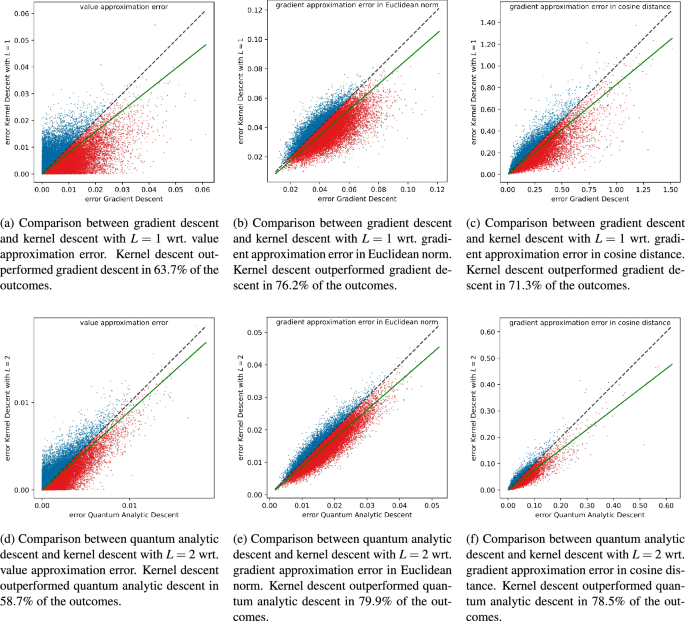

This figure shows the scatter plots of the first type from Sect. 3.2. Points below the diagonal (colored red) correspond to outcomes where kernel descent outperformed the algorithm it was being compared to. The green line is the line through the origin, whose polar angle is the average of the polar angles of the $N = 25,000$ points appearing in the scatter plot. The fact that the green lines are running below the diagonals is a further indication that kernel descent outperformed the algorithm it was being compared to; see Sect. 3.2 for details.

Figure 4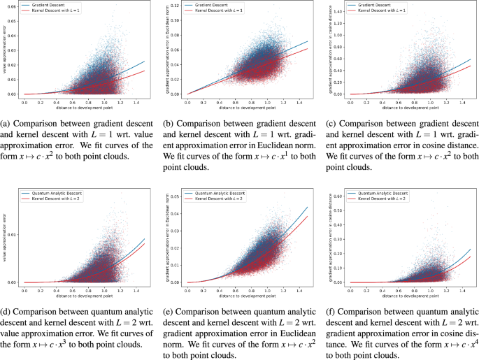

This figure shows the scatter plots of the second type from Sect. 3.2. The red curve running below the blue curve indicates that kernel descent outperformed the algorithm it was being compared to; see Sect. 3.2 for details.

Performance of the algorithms

Here we compare the algorithms with respect to their ability to minimize the objective function. The comparisons of kernel descent with $L=1$ versus gradient descent and kernel descent with $L=2$ versus quantum analytic descent follow a similar pattern, albeit with some key differences which are imposed by the higher computational demands per iteration of the second pair of algorithms.

Kernel descent versus gradient descent

To level the playing field, we carry out kernel descent with $L=1$ and gradient descent in their most basic form without specialized enhancements such as learning rate adaptation. In particular, we assume that gradient descent operates with a fixed learning rate $\alpha >0$. Moreover, we rescale the steps of the inner optimization loop of kernel descent so that their combined length equals that of the corresponding gradient descent step. We will now describe the experiments in detail and then conclude with our observations.

Circuit sampling and running the algorithms

In order to keep the computational load manageable, we set $n=m=8$ and choose $T=20$ iterations per algorithm. We will compare the algorithms using $N=5,000$ randomly sampled circuits, and for each circuit we will test three different learning rates $\alpha _1 =7.0$, $\alpha _2 =8.5$ and $\alpha _3 =10.0$. Each of the $N=5,000$ test runs will follow the scheme outlined below.

1.

Circuit sampling: A circuit, an initial point $\theta _0\in \mathbb {R}^m$ and an observable $\mathcal {M}$ are sampled randomly as explained in Sect. 3.1, and f is defined as in Sect. 2.1.
2.

Gradient descent runs: Starting from initial point $\theta _0$, gradient descent with $T=20$ steps is executed three times with the three different learning rates: $\alpha _1$,$\alpha _2$ and $\alpha _3$. This yields three sequences of points in parameter space which we denote by

$$\Theta ^{\operatorname {GD}}_i\,:=\,\Theta ^{(\operatorname {GD}, \alpha _i)}\,:=\, \left( \theta _{0}, \theta _{1}^{(\operatorname {GD}, \alpha _i)}, \dots , \theta _{20}^{(\operatorname {GD}, \alpha _i)}\right) ,$$

where $i=1,2,3$.
3.

Kernel descent runs: Starting from initial point $\theta _0$, kernel descent with $L=1$ and $T=20$ steps is executed three times:
- Denote the current point in parameter space after t iterations of kernel descent by $\theta _t$, and the local approximation of f around $\theta _t$ by $\tilde{f}_t$. In the inner optimization loop we execute $k=100$ gradient descent steps with respect to $\tilde{f}_t$.
- In the three executions of kernel descent, the learning rates for the inner optimization loops are $\alpha _1 / k = 0.07$, $\alpha _2 / k = 0.085$ and $\alpha _3 / k = 0.1$. This rescaling of the learning rates accounts for the number of gradient descent steps taken in the inner loop.
- At each of the k gradient descent steps of the inner optimization loop starting at $\theta _t$, the gradient of the local approximation $\tilde{f}_t$ is rescaled to have length $\Vert \nabla f (\theta _t)\Vert$ (numerical instability and division by 0 are prevented by adding a small positive constant to the occurring denominators). Since $\nabla f (\theta _t) = \nabla \tilde{f}_t (\theta _t)$ by Theorem 3(iii), computation of $\nabla f (\theta _t)$ does not require any additional circuit evaluations.
We thus obtain three sequences of points in parameter space, one per learning rate, which we denote by

$$\Theta ^{\operatorname {KD}}_i\,:=\,\Theta ^{(\operatorname {KD}, \alpha _i)}\,:=\,\left( \theta _{0}, \theta _{1}^{(\operatorname {KD}, \alpha _i)}, \dots , \theta _{20}^{(\operatorname {KD}, \alpha _i)}\right) ,$$

where $i=1,2,3$.

The final outcome of this procedure is a family

$$\Theta :=\,\left( \Theta ^{\operatorname {A}}_i\right) _{\operatorname {A}\in \{\operatorname {GD}, \operatorname {KD}\},i\in \{1,2,3\}}$$

of six point sequences in parameter space—one per combination of algorithm and learning rate—for each of the $N=5,000$ randomly sampled circuits.

Normalization

Since the circuit, initial point, and observable were sampled randomly in each of the $N=5,000$ test runs, we cannot directly compare the values of the objective function f between different runs. We remedy this by normalizing the f-values of the point sequences we computed. Specifically, for each of the $N=5,000$ families $\Theta$, the following is carried out: Let v be the minimal value of f attained at a point in any of the sequences in $\Theta$. That is, $v = \min (\{f(\theta _{0}),f(\theta _{t}^{(\operatorname {GD}, \alpha _i)}), f(\theta _{t}^{(\operatorname {KD}, \alpha _i)}) | t\in \{1,\dots , 20\} , i\in \{1,2,3\}\}).$ In the pathological case where v is not smaller than $f(\theta _0)$, one would discard the family $\Theta$ and compute another one. However, this did not happen in our experiments. Now let

$$\begin{aligned} \ell :\mathbb {R}\rightarrow \mathbb {R},\ x\mapsto \tfrac{x-v}{f(\theta _0)-v} \end{aligned}$$

(3)

be the uniquely determined affine linear map that maps $f(\theta _0)$ to 1 and v to 0. Applying $\ell$ component-wise to the sequences of f-values corresponding to the point sequences in $\Theta$, we obtain three normalized sequences for gradient descent,

$$\begin{aligned} \bar{f}_i^{\operatorname {GD}}\,:=\,\left( 1, \ell (f(\theta _{1}^{(\operatorname {GD}, \alpha _i)})) , \dots , \ell (f(\theta _{20}^{(\operatorname {GD}, \alpha _i)}))\right) , \end{aligned}$$

and three normalized sequences for kernel descent,

$$\begin{aligned} \bar{f}_i^{\operatorname {KD}}\,:=\,\left( 1, \ell (f(\theta _{1}^{(\operatorname {KD}, \alpha _i)})) , \dots , \ell (f(\theta _{20}^{(\operatorname {KD}, \alpha _i)}))\right) , \end{aligned}$$

where $i=1,2,3$.

Illustration and observations

For a fixed learning rate $\alpha _i$, where $i\in \{1,2,3\}$, and a fixed algorithm $\operatorname {A}\in \{\operatorname {GD}, \operatorname {KD}\}$ we can obtain an averaged sequence of normalized f-values by taking the component-wise average over all $N=5,000$ normalized sequences $\bar{f}^{\operatorname {A}}_i$. The so-obtained sequence can be interpreted as the average performance of the considered combination of algorithm and learning rate. Comparisons of these average performances are visualized in Fig. 5.

Upon closer inspection we realized that, for the smallest learning rate $\alpha _1$, the direction of the true gradient vector did typically not change by much between two consecutive gradient descent steps. Because of this, and since we ensured that the length of the path in parameter space traversed during the inner optimization loop of kernel descent equals the length of the corresponding gradient descent step, one cannot expect kernel descent with $L=1$ to significantly outperform gradient descent at learning rate $\alpha _1$ in our experiments. Nevertheless, as the quality of the local approximations computed by kernel descent with $L=1$ is typically higher than the quality of the best linear approximation (see Sect. 3.2), kernel descent with $L=1$ can still be expected to perform slightly better than gradient descent, even at small learning rates. These expectations are confirmed in Fig. 5a.

For the largest learning rate, $\alpha _3$, the steps taken by gradient descent were often too large and the algorithm did not converge. Contrary to this, in the inner optimization loop of the corresponding execution of kernel descent with $L=1$, the descent often got caught in a local minimum of the local approximation, which effectively prevented the algorithm from moving away too far from the development point. As a result, kernel descent typically converged, while gradient descent typically did not. This is mirrored in Fig. 5c.

For learning rate $\alpha _2$, we observed a mixture of the phenomena which we observed for learning rates $\alpha _1$ and $\alpha _3$. Non-surprisingly, the robustness advantages of kernel descent (against taking exceedingly large steps in parameter space) were less pronounced than with learning rate $\alpha _3$, while the advantages in terms of speed of descent (owing to the better approximation quality, see Sect. 3.2) were more pronounced than with learning rate $\alpha _1$. The results for learning rate $\alpha _2$ are visualized in Fig. 5b.

Out of all six combinations of algorithm and learning rate, kernel descent with $L=1$ and learning rate $\alpha _3$ performed the best in our experiments. Moreover, every combination involving kernel descent performed better than all combinations involving gradient descent, see Fig. 5d–f.

In conclusion, kernel descent with $L=1$ outperformed gradient descent at small learning rates in our experiments, which we ascribe to the higher quality of the local approximations, see Sect. 3.2. Moreover, kernel descent with $L=1$ was more robust with respect to the choice of learning rate, which we ascribe to the presence of local minima for the local approximations computed during kernel descent with $L=1$. While the local approximations computed during kernel descent necessarily have local (and global) minima, it is not clear whether the robustness effect we observed in our experiments will continue to hold outside of our experimental setup. An investigation of the latter is left for future work.

Figure 5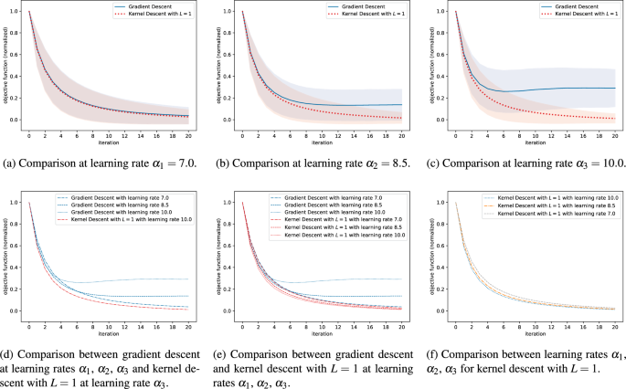

This figure shows the performance of gradient descent and kernel descent with $L=1$ for three different learning rates, averaged over $N=5,000$ respective executions. In each execution, the circuit, observable and initial point in parameter space were sampled randomly. Consequently, for the sake of comparability, we introduced a normalization step before averaging; see Sect. 3.3 for details. In Fig. 5a–c we compare gradient descent to kernel descent with $L=1$ at learning rates $\alpha _1 =7.0$, $\alpha _2 =8.5$ and $\alpha _3 =10.0$ respectively; we also indicate the respective standard deviations. In Fig. 5d–f we make comparisons between different learning rates.

Kernel descent versus quantum analytic descent

The comparison of kernel descent with $L=2$ versus quantum analytic descent follows a similar scheme as the comparison of kernel descent with $L=1$ versus gradient descent. Key differences concern the random sampling of the observable and the stopping criteria for the inner optimization loops of the algorithms.

Circuit sampling

The circuit and the initial point in parameter space are sampled precisely as described in Sect. 3.1. The observable $\mathcal {M}$ is sampled as follows: We randomly sample (independently) twenty n-qubit Paulis $\mathcal {P}_1, \dots , \mathcal {P}_{20}$ from the uniform distribution on $\{I,X,Y,Z\}^{\otimes n}$; we also randomly sample (independently) coefficients $c_1, \dots , c_{20}$ from the standard normal distribution. We then set $\mathcal {M}:=\sum _{i=1}^{20}c_i\mathcal {P}_i$.

The inner optimization loop

To ensure a fair comparison, the inner optimization loop was conducted in the same way for kernel descent and quantum analytic descent; specifically, we used gradient descent with learning rate 0.01 and applied the same stopping criterion to both algorithms. In order to be as impartial as possible, we used one of the stopping criteria given in the original work on quantum analytic descent25:

The inner optimization loop is stopped as soon as the true value of f is increased. Since every determination of the true value of f requires an additional circuit evaluation, we only determine the true value of f every $1000^\text {th}$ step of the inner loop. Moreover, in order to prevent an infinite loop and to upper-bound the number of circuit evaluations per iteration of the algorithms, we set an upper bound of 10000 steps after which the inner optimization loop is aborted, even if the true value of f has not been found to increase. Consequently, at most 9 additional circuit evaluations are incurred as a result of the inner optimization loop—which is negligible in comparison to the overall number of circuit evaluations per iteration.

Experiment execution

Due to the aforementioned higher computational cost per iteration the number of test runs for the current comparison is reduced from $N=5,000$ to $N=500$. In each run the following is performed:

1.

A circuit, an initial point $\theta _0\in \mathbb {R}^m$ and an observable $\mathcal {M}$ are sampled randomly as explained previously.
2.

Starting from initial point $\theta _0$, both quantum analytic descent and kernel descent with $L=2$ are executed each with $T=5$ steps (with inner optimization loop as described above). We denote the resulting sequences of points in parameter space by

$$\Theta ^{\operatorname {QAD}}\,:=\,\left( \theta _{0}, \theta _{1}^{(\operatorname {QAD)}}, \dots , \theta _{5}^{(\operatorname {QAD})}\right)$$

and

$$\Theta ^{\operatorname {KD}}\,:=\,\left( \theta _{0}, \theta _{1}^{(\operatorname {KD})}, \dots , \theta _{5}^{(\operatorname {KD})}\right) \,,$$

respectively.

Normalization

As in Sect. 3.3 we need to introduce a normalization step before we can compare the values of the objective function f between different runs. For each of the $N=500$ runs we proceed as follows: We denote the minimal value of f attained during execution of the two algorithms by v. That is,

$$v = \min (\{f(\theta _0 ), f(\theta _{t}^{(\operatorname {QAD})}), f(\theta _{t}^{(\operatorname {KD})}) | t\in \{1,\dots , 5\}\}).$$

As above, no pathological cases (where $v=f(\theta _0)$) arose and thus no exception handling was necessary.

Using v, we define $\ell : \mathbb {R}\rightarrow \mathbb {R}$ as in (3). Applying $\ell$ component-wise to the sequences of values obtained during execution of the algorithms, we obtain normalized sequences

$$\begin{aligned} \bar{f}^{\operatorname {QAD}}\,:=\,\left( 1, \ell (f(\theta _{1}^{(\operatorname {QAD})})) , \dots , \ell (f(\theta _{5}^{(\operatorname {QAD})}))\right) , \end{aligned}$$

and

$$\begin{aligned} \bar{f}^{\operatorname {KD}}\,:=\,\left( 1, \ell (f(\theta _{1}^{(\operatorname {KD})})) , \dots , \ell (f(\theta _{5}^{(\operatorname {KD})}))\right) \,. \end{aligned}$$

As in Sect. 3.3, we then compute the component-wise average of the $N=500$ normalized sequences $\bar{f}^{\operatorname {QAD}}$ (resp. $\bar{f}^{\operatorname {KD}}$).

Results

Kernel descent with $L=2$ clearly outperformed quantum analytic descent, in the sense that the average curve for kernel descent runs below that of quantum analytic descent, see Fig. 6.

Figure 6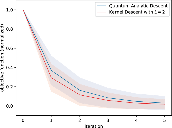

This figure shows the performance of quantum analytic descent and kernel descent with $L=2$ averaged over $N = 500$ respective executions. In each execution, the circuit, observable and initial point in parameter space were sampled randomly. Consequently, for the sake of comparability, we introduced a normalization step before averaging; see Sect. 3.3 for details. We also indicate the respective standard deviations.

Experiment with 8-qubit spin ring Hamiltonian

The first part of Sect. 3, described in Sects. 3.1, 3.2, and 3.3, was concerned with a large number of randomized circuits and observables. Here, in the second part, we experimentally compare the performance of gradient descent and kernel descent with $L=1$ for an observable and a circuit that are more representative of real world applications.

The problem

We address the problem of finding the ground state energy of an 8-qubit spin ring Hamiltonian, which was already investigated in25. Specifically, we consider the Hamiltonian

$$\sum _{i=1}^{8} 0.1\cdot (X_i X_{i+1} + Y_i Y_{i+1} + Z_i Z_{i+1}) + \sum _{i=1}^{8} \omega _i Z_i,$$

where all indices are taken modulo 8 with system of representatives $\{1,2,\dots , 8\}$, and $\omega _1,\dots , \omega _8\in [-1,1]$ were independently sampled uniformly at random.

Ansatz circuit

We adopt the ansatz circuit from25, i.e., starting with $n=8$ qubits in state $|0\rangle ^{\otimes 8}$, we apply a parametrized $R_X$ gate to every qubit and subsequently apply four consecutive blocks, each consisting of

1.

parametrized $R_{ZZ}$ gates, applied to qubit pairs (7, 8), (6, 7), (5, 6), (4, 5), (3, 4), (2, 3), (1, 2), and (8, 1),
2.

followed by parametrized $R_Y$ gates applied to every qubit,
3.

followed by parametrized $R_X$ gates applied to every qubit.

In particular, we have $m=8+4\cdot (8+8+8) = 104$. The circuit is visualized in Fig. 7.

Figure 7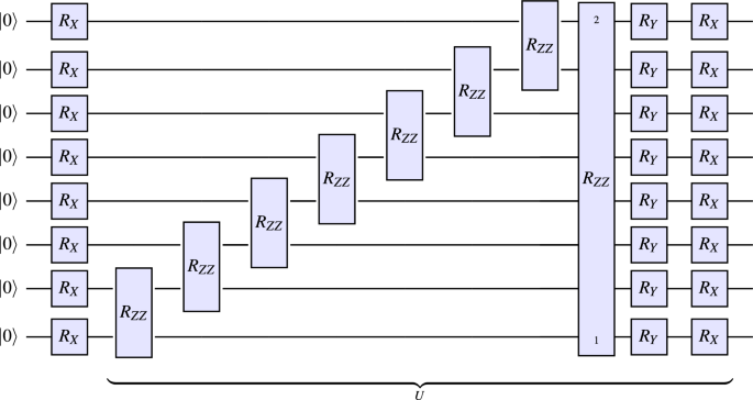

This figure shows the ansatz circuit used for the experiments in Sect. 3.4. While, for clarity, the U-block is depicted only once, the circuit consists of an initial layer of parametrized $R_X$ gates and four consecutive U-blocks (with different parameters, i.e., we are not re-uploading parameters). In particular, the ansatz circuit has $m=8+4\cdot (8+8+8)=104$ parameters.

Experiment execution

All circuit evaluations were executed using 1000 measurement shots. After sampling an initial point in parameter space from the uniform distribution on $[-\pi ,\pi )^{104}$, both gradient descent and kernel descent with $L=1$ were executed $N=100$ times, with 30 iterations per execution, yielding $N=100$ respective sequences in parameter space of length 31 (including the initial point). For each such sequence in parameter space we then determined the corresponding sequence of true values of the objective function f using statevector simulation (exact evaluations of f did not have an impact on the execution of either algorithm, but were only used to compare the results). Subsequently, for both algorithms, we computed the component-wise average of the $N=100$ sequences of values to get an indication of their respective average performance. However, since the stopping criterion for kernel descent we used in this experiment incurs additional circuit evaluations in the inner optimization loop (see below), we compare the performance of the algorithms based on the number of executed measurement shots. Since, when using the above-mentioned stopping criterion for the inner optimization loop, the number of measurement shots per iteration of kernel descent is not constant, we also averaged the cumulative number of measurement shots for each of the 30 iterations over the $N=100$ executions of kernel descent.

Gradient descent

The learning rate for gradient descent was 0.3 (the largest learning rate under which stable behavior was observed), and gradients were evaluated using the parameter-shift rules with $\pm \frac{\pi }{2}$-shifts.

Kernel descent with $L=1$

We employed a similar stopping criterion for the inner optimization loop as in Sect. 3.3. Specifically, we used gradient descent with learning rate 0.001 in the inner optimization loop and terminated the inner optimization loop as soon as the value of f was increased; the value of f (up to shot noise) was determined every $100^\text {th}$ step of the inner loop and we set an upper bound of 5000 steps for the inner loop, after which the loop was aborted even if the value of f was not found to increase. The upside of using this stopping criterion is that one can forego a (potentially lengthy) tuning process for the hyperparameters of the inner optimization loop. The downside is that this stopping criterion incurs several additional circuit evaluations in each iteration of the outer optimization loop. In order to not give kernel descent an unfair advantage over gradient descent (the additional circuit evaluations), we compare the performance of the algorithms based on the number of executed measurement shots (and not based on the number of executed iterations), see above.

Results

Kernel descent with $L = 1$ clearly outperformed gradient descent, in the sense that the average curve for kernel descent runs below that of gradient descent, see Fig. 8.

Figure 8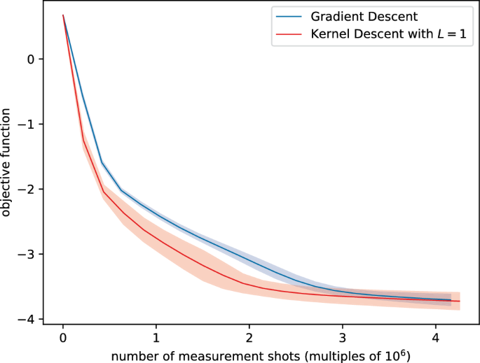

This figure shows the performance (under the presence of measurement shot noise) of gradient descent and kernel descent with $L=1$ in finding the ground state energy of an 8-qubit spin ring Hamiltonian, averaged over 100 respective executions. Since the stopping criterion we used for the inner optimization loop of kernel descent incurs additional circuit evaluations, we compare the performance of the algorithms based on the number of executed measurement shots; see Sect. 3.4 for details. We also indicate the respective standard deviations.

Introducing the kernel descent optimizer for variational quantum algorithms

Tags: