Figure 1 a illustrates the 3D microwave cavities used in our system, each with four ports featuring adjustable coupling rates, tunable (identical) resonance frequency, ωc, and fixed internal loss rates, κint. Figure 1b presents an exploded view of the cavities, showing the length-adjustable couplers, each formed by the center conductor of a coaxial connector that controls the input, output, and coupling rates, labeled as κin, κout, and κc, respectively. The resonance frequency is tuned by adjusting a post at the base of the device, with locking pins ensuring the stability of all mechanically-tunable parameters after calibration.
Fig. 1: Tunable, non-Hermitian, nonlinear microwave dimer.
a Depiction of individual cavities with a mechanically-adjustable resonance frequency and coupling rates. b An exploded view of the cavity, showing how cavities are assembled with locking pins to set experimental parameters after calibration. c Schematic of the dimer system formed from two tunable microwave harmonic oscillators with frequencies ωc/2π = 6.027(5) GHz and internal quality factors of Qint = ωc/κint ≈ 1488. The oscillators are connected with a characteristic coupling strength of κc/2π = 8.7(1) MHz. When the amplifier is in its normal operating regime, this coupling is determined by a characteristic gain, G0 = 20.3(2) dB, and subsequently adjusted through digital attenuation, Γ. On the return path (cavity 2 → cavity 1), a phase shifter introduces a relative phase, ϕ, between the two coupling paths. We couple photons into and out of the cavity at an average rate κin,out/2π = 4.0(2) MHz.
As shown in Fig. 1c, cavity 1 is driven by a coherent signal with strength ϵ and frequency ωd at an input rate κin. Hence, we define \(\epsilon \equiv \sqrt{{\kappa }_{{{{\rm{in}}}}}{P}_{{{{\rm{in}}}}}/\hslash {\omega }_{d}}\), where Pin is the input drive power (in watts), converted from the corresponding value Pd (in dBm) using \({P}_{{{{\rm{in}}}}}=1{0}^{({P}_{d}-30)/10}\).
Both cavities are coupled to unidirectional amplifiers with a characteristic gain G0, followed by a digital attenuator with a dynamic range of Γ ∈ [0, 50] dB, adding to the intrinsic insertion loss of the passive components. A digital phase shifter is inserted to make the relative phase, ϕ, of the reverse propagating path (cavity 2 → cavity 1) tunable over [0, 2π), and the output is collected from cavity 2 at a rate κout. In what follows, we characterize our system using the quantity ΔG ≡ G0 − Γ, representing the net hopping gain. By utilizing a conversion factor of 10ΔG/20, we adjust the intrinsic κc of each oscillator to produce an effective, tunable hopping coefficient at low power given by J0(ΔG) = 10ΔG/20κc.
Before describing the full nonlinear model of our system, we present a linear model that accurately describes the essential features of the dynamics in the low-power regime. This is achieved by considering the following semiclassical equations of motion (EOMs):
$$\dot{{{\alpha }}}={A}_{0}{{\alpha }}+\epsilon {{{\rm{B}}}},$$
(1)
where the state variables \({{\alpha }}\equiv {\left[\begin{array}{c}{\alpha }_{1}{\alpha }_{2}\end{array}\right]}^{T}\) represent complex amplitudes of the cavity field, \({{{\rm{B}}}}\equiv {\left[\begin{array}{c}10\end{array}\right]}^{T}\) accounts for the external drive on cavity 1, and the dynamical matrix A0 takes the form
$${A}_{0}=\left[\begin{array}{cc}-i({\omega }_{c}-{\omega }_{d})-{\kappa }_{0}&-i{J}_{0}(\Delta G){e}^{-i\phi }\hfill \\ -i{J}_{0}(\Delta G)\hfill &-i({\omega }_{c}-{\omega }_{d})-{\kappa }_{0}\end{array}\right].$$
(2)
In this way, tuning the phase ϕ takes the system from a regime where the hopping dynamics is perfectly reciprocal (ϕ = 0), to one where the couplings are skew-Hermitian (ϕ = π). Thus, phase non-reciprocity occurs in our system when the relative phase of the hopping terms differ, despite the hopping rates remaining equal. As a key difference from existing non-reciprocal devices, our dynamical matrix A0 is non-Hermitian but nonetheless normal (hence diagonalizable) throughout the undriven parameter regime.
In Eq. (2), we have introduced the parameter κ0 to describe the total intra-cavity dissipation rate. Experimental observations suggest that κ0 is also influenced by J0(ΔG). This influence can be explained by the increase in state amplitudes within the cavities, αi, which leads to the amplifiers introducing and amplifying existing incoherent noise over a finite bandwidth determined by the inherent linewidth of the cavities. Since this amplified noise competes directly with the intrinsic dissipation of each cavity, the overall effective dissipation rate is reduced. We model this process phenomenologically as:
$${\kappa }_{0}\equiv {\kappa }_{0}(\Delta G)=2\,({\kappa }_{{{{\rm{int}}}}}+{\kappa }_{{{{\rm{in}}}}/{{{\rm{out}}}}}+{\kappa }_{c})-{J}_{0}(\Delta G).$$
(3)
Generally, Eq. (1) admits a unique stable equilibrium point when \(\max {{\rm{Re}}}\,[\sigma ({A}_{0})] , where σ(A0) ≡ σ(A0(ΔG, ϕ)) denotes the eigenvalue spectrum of A0 as a function of the tunable parameters. Thus, a necessary and sufficient condition for dynamical stability is that
$$\frac{{J}_{0}(\Delta G)}{{\kappa }_{0}(\Delta G)}\sin (\phi /2)
(4)
The associated stability phase boundary as a function of ϕ and ΔG is illustrated in Fig. 2a. From Eq. (4), we can immediately see that for ϕ ≠ 0 and sufficiently high ΔG, it is possible that J0(ΔG) can balance and exceed κ0(ΔG), resulting in the onset of instability. This condition selects two relevant regions, namely,
$$\,{{\rm{Region I:}}}\,0\le {J}_{0}(\Delta G)\le {\kappa }_{0}(\Delta G),$$
(5)
$$\,{{\rm{Region II:}}}\,{\kappa }_{0}(\Delta G)
(6)
Region I is always stable, while Region II is only stable for those ϕ satisfying Eq. (4). Physically, in the gain-dominated (Region II) unstable regime, the field amplitudes ∣αi∣2 diverge, pushing the amplifiers into saturation and reducing the gain in a power-dependent fashion.
Fig. 2: Stability phase diagram and transmission spectra (S21) for our tunable non-Hermitian nonlinear microwave dimer.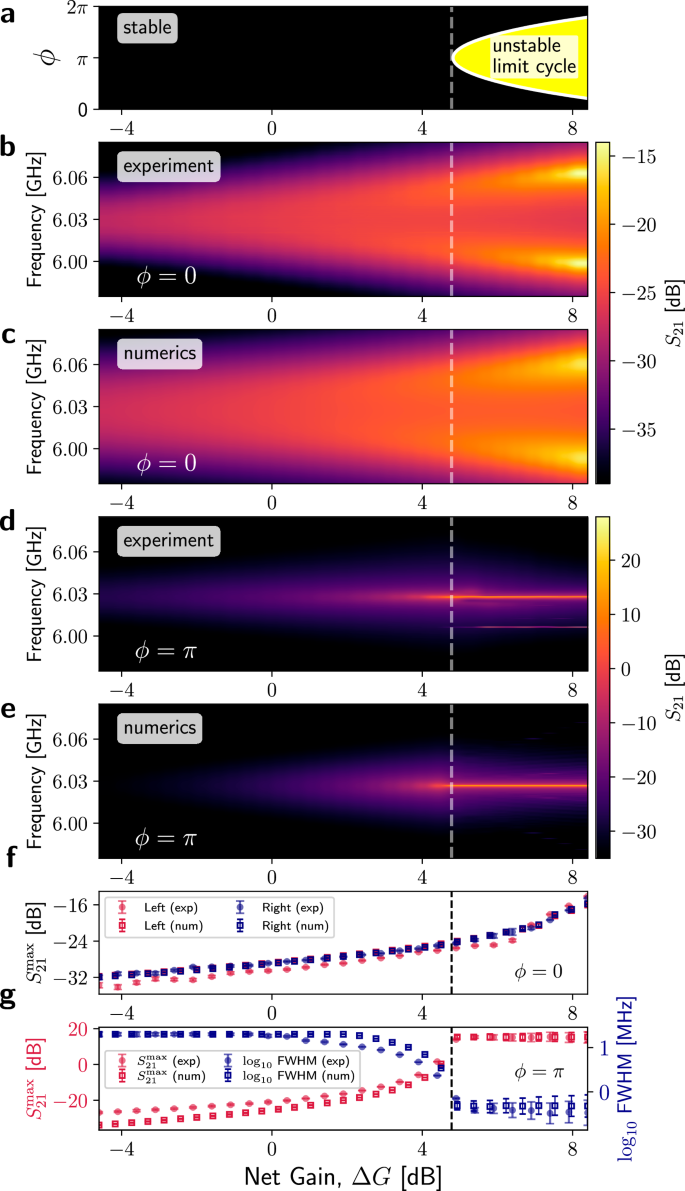
a Stability phase diagram depicting the vacuum-stable and unstable regimes determined by the dynamical matrix in Eq. (2) or Eq. (9). b(d), Experimental, and c(e) numerical simulations for S21 as a function of net gain, ΔG, for ϕ = 0(π). In both cases, data are plotted with the same colorbar for direct comparison. Numerical simulations (squares) and experimental measurements (circles) of maximum transmission, \({S}_{21}^{\max }\), are shown in (f) and (g). A comparison of the experimental full width at half maximum (FWHM) with corresponding numerical results for ϕ = π is included in (g), showing a dramatic reduction in linewidth as ΔG increases. \({S}_{21}^{\max }\) and FWHM are extracted from single- or double-Lorentzian fits to the spectra in b-c and d-e, with error bars indicating one standard deviation from the fit covariance matrix. FWHM is shown on a logarithmic scale to highlight the sharp transition to sub-MHz linewidths above threshold. Experimental and numerical results in (b)–(g) consider an input drive power of Pd = − 30 dBm. The dashed line at ΔG = 4.78 in a-g denotes the onset of instability at ϕ = π.
While the linear model captures the correct asymptotic behavior in the stable, loss-dominated (Region I) regime, to obtain a description of the dynamical behavior valid in both the above regions, we must allow the hopping function to depend nonlinearly upon ∣αi∣2. We account for such a dependence through the following continuous piecewise function:
$$\frac{J(\Delta G;| {\alpha }_{i}{| }^{2})}{{\kappa }_{c}1{0}^{\Delta G/20}}=\left\{\begin{array}{ll}1\hfill \quad &\,{{\rm{if}}}\,\,| {\alpha }_{i}{| }^{2}\le | {\alpha }_{{{{\rm{sat}}}}}{| }^{2},\\ \frac{{b}_{G}+\hslash {\omega }_{c}| {\alpha }_{{{{\rm{sat}}}}}{| }^{2}{\kappa }_{c}}{{b}_{G}+\hslash {\omega }_{c}| {\alpha }_{i}{| }^{2}{\kappa }_{c}}\quad &\,{{\rm{if}}}\,\,| {\alpha }_{i}{| }^{2} > | {\alpha }_{{{{\rm{sat}}}}}{| }^{2},\end{array}\right.$$
(7)
where bG = 8.6 mW and ∣αsat∣2 is the saturation threshold of the amplifier, which is determined by ∣αsat∣2 = Psat/ℏωcκc, with Psat = 0.9981 mW derived from experimental characterization (see Supplementary Information Sec. VI). Note that for sufficiently low ∣αi∣2, Eq. (7) consistently recovers the hopping coefficient for the linear model, namely J0(ΔG). However, as ∣αi∣2 exceeds ∣αsat∣2, J(ΔG, ∣αi∣2) becomes monotonically reduced, illustrating the saturation effect that drives the nonlinear behavior of the system.
As we will further discuss in the next section, transmission experiments (Fig. 2b,d) show that peak-splitting at ϕ = 0 is first resolved at a significantly lowerΔG than the one at which instability sets in for ϕ = π. However, Eq. (2) indicates that the two normal modes become spectrally resolvable, namely when their splitting equals the peak linewidth, only at ΔG ≃ 4.78 dB, so it predicts that the resolvable splitting and the instability threshold should coincide. This suggests an additional coherent hopping effect that is stronger at ϕ = 0, allowing for earlier mode splitting (see also Supplementary Information, Sec. IB). We make this intuition precise by directly modifying the off-diagonal hopping coefficients via a phase-dependent function, \(f(\phi )=i{J}_{c}\cos \left(\frac{\phi }{2}\right){e}^{i\phi /2},\) where Jc/2π = 11.5 MHz represents the strength of this additional coherent hopping. While a complete explanation of the origin of f(ϕ) is lacking, and its proposed ϕ-dependence is phenomenological, we believe it stems from constructive interference between the two modes. The incorporation of f(ϕ) accurately captures the frequency splitting observed in Fig. 2b–e without altering the stability characteristics of the system in Fig. 2a.
At this point, we have already introduced all of the terms required to define the final form of our EOMs:
$$\dot{{{\alpha }}}=A(| {\alpha }_{1}{| }^{2},| {\alpha }_{2}{| }^{2}){{\alpha }}+\epsilon {{{\rm{B}}}},$$
(8)
with the full dynamical matrix being given by
$$ A(| {\alpha }_{1}{| }^{2},| {\alpha }_{2}{| }^{2})\\ =\left[\begin{array}{cc}-i({\omega }_{c}-{\omega }_{d})-{\kappa }_{1}(\Delta G;| {\alpha }_{1}{| }^{2})&[-iJ(\Delta G;| {\alpha }_{2}{| }^{2})-f(\phi )]{e}^{-i\phi }\\ -iJ(\Delta G;| \alpha {| }_{1}^{2})-f(\phi )\hfill &-i({\omega }_{c}-{\omega }_{d})-{\kappa }_{2}(\Delta G;| {\alpha }_{2}{| }^{2})\end{array}\right],$$
(9)
where κ1(2) = 2(κint,1(2) + κin(out) + κc) − J(ΔG, ∣α1(2)∣2), and J(ΔG, ∣α1(2)∣2) is defined in Eq.(7). In the linear limit of small ∣αi∣2, A(∣α1∣2, ∣α2∣2) reduces to A0 as described in Eq.(2), up to the phase-dependent correction introduced via f(ϕ). By explicitly solving the dynamics defined by Eqs. (8) and (9), we can directly reproduce and capture the main features observed in our experiments, such as weak-drive transmission (Fig. 2b–g), undriven LC solutions (Figs. 2a and 3), as well as the phase locking synchronization phenomena (Fig. 4). We provide an in-depth discussion in the sections that follow.
Fig. 3: Phase diagram of the amplitude and frequency of the LC solutions without external driving.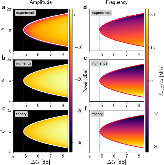
a–c Power emitted from the LC extracted experimentally (a), numerically (b), and analytically (c). d–f Frequency detuning of the LC relative to ωc, δωLC, extracted experimentally (d), numerically (e), and analytically (f). The contour in each plot represents the stability phase boundary from the dynamical matrix in Eq. (9), also corresponding to ∣α2∣2 = ∣αsat∣2 for the analytical solution in Eq. (10), which is depicted in (c) and (f). Numerical and analytical amplitudes in the vacuum-stable phase in (b)–(c) are set at -44 dBm, corresponding to the baseline amplitude observed experimentally in a, and this same threshold is used to white out the corresponding region in (d). The vertical dashed line in all plots marks the value of net gain ΔG = 4.78 dB at which the phase ϕ = π becomes unstable. In the experimental data, we removed an outlier near ϕ = 5.287 rads., corresponding to the set value on the digital phase shifter moving from 2π → 0.
Fig. 4: Synchronization of the LC mode and an external drive.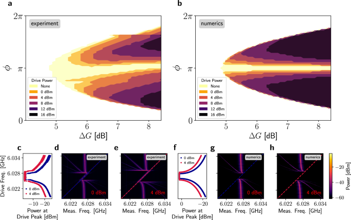
Experimental (a) and numerical (b) contours representing regions containing a distinct LC away from ωc/2π as a function of drive power. For the experimental and numerical data presented in (a) and (b), we applied an external drive at ωd/2π = ωc/2π = 6.027 GHz. Note that in the LC region of a and b, if ϕ = π, then ωc = ωd = ωLC, whereas for ϕ ≠ π, we have ωc = ωd ≠ ωLC. Experimental (c) and numerical (f) power of the drive peak as a function of the drive frequency for the panels presented in (d)–(e) and (g)–(h) depicted as blue and red dashed lines for Pd = 0 and 4 dBm, respectively. Experimental (d–e) and numerical (g–h) emission from the dimer at ϕ = π and ΔG = 8.4 dB as an external drive is swept from low to high frequency around ωc/2π for Pd = 0 dBm (d, g), and for Pd = 4 dBm (e, h) drive strengths, showing mixing and phase locking synchronization with the external drive. In both experimental and numerical simulations, the LC synchronizes in a larger range in frequency as Pd increases, consistent with the expansion of synchronized regions shown in c and f, which explains the trend observed in the vicinity of ϕ = π for the contours depicted in (a)–(b), respectively.
Weak-drive transmission spectra
To probe the steady-state S21, we drive the system at an input power of Pd = − 30 dBm and sweep the drive frequency ωd/2π over the range 5.98 to 6.09 GHz using a scalar network analyzer. Numerically, we compute S21 as the ratio of the steady-state output power from cavity 2 and the input drive power in cavity 1. Hence,
$${S}_{21}({\omega }_{d},\Delta G,\phi )=\frac{{P}_{{{{\rm{out}}}}}}{{P}_{{{{\rm{in}}}}}}=\frac{\hslash {\omega }_{d}{\left\vert {\alpha }_{2}^{{{{\rm{eq}}}}}\right\vert }^{2}{\kappa }_{{{{\rm{out}}}}}}{\hslash {\omega }_{d}{\epsilon }^{2}/{\kappa }_{{{{\rm{in}}}}}}={\kappa }_{{{{\rm{in}}}}}{\kappa }_{{{{\rm{out}}}}}\frac{{\left\vert {\alpha }_{2}^{{{{\rm{eq}}}}}\right\vert }^{2}}{{\epsilon }^{2}},$$
where \({\alpha }_{2}^{{{{\rm{eq}}}}}\) is the DC-component of the unique asymptotic solution α2(t). Note that the dependence on ΔG and ϕ is implicitly contained in the solutions for \({\alpha }_{2}^{{{{\rm{eq}}}}}\). Moreover, to directly compare numerical solutions to experimental results, the conversion to dB is accomplished via S21 [dB] \(=10{\log }_{{{{\rm{10}}}}}({S}_{21})\).
Figure 2b–g present the experimental and numerical S21 data for the two special phases, ϕ = 0 and ϕ = π, for which, as noted, the hopping amplitudes are Hermitian and skew-Hermitian, respectively. Specifically, Fig. 2b–c depict the experimental and numerical S21 spectra for ϕ = 0 across various ΔG values. At low ΔG, the S21 spectra show a single, very broad peak, indicating that the two modes are decoupled due to the high effective loss in the hopping path. As ΔG increases, two distinct peaks emerge and move further apart, demonstrating enhanced coupling and symmetric energy distribution between the two modes. The increasing separation of the peaks and higher S21 magnitudes (indicated by brighter colors at higher ΔG in Fig. 2b–c) confirm the successful experimental implementation of reciprocal hopping with tunable rates, as predicted by the dynamical matrix in Eq. (9) at ϕ = 0. Additionally, the excellent agreement between experimental results and numerical simulations presented in Fig. 2b–c validates the accuracy of our model by capturing the S21 characteristics when the coupling coefficients in both paths are engineered to be nominally equal.
Figure 2d–e show the experimental and numerical S21 spectra at ϕ = π. At low ΔG values, we observe a minimal S21 signal, again indicating that the two modes are essentially decoupled. As ΔG increases to intermediate levels, the signal response increases, but the transmission spectra differ significantly from the typical frequency splitting seen in symmetrically coupled modes. Instead of two peaks in frequency, we observe a single peak centered at ωc/2π. When ΔG ≃ 4.78 dB and beyond, the amplitude of the peak at ωd ≃ ωc suddenly and dramatically increases, followed by asymptotic saturation, while its linewidth sharply narrows (Fig. 2g), consistent with the onset of a stable LC.
Since the scalar network analyzer performs homodyne detection at the drive frequency, the experimental S21 measurements effectively collect the steady-state transmission amplitude at ωd/2π. We account for this effect into our numerical framework to generate the data presented in Fig. 2 by breaking down the time-domain signal into its frequency components and extracting the DC component, as described in the Methods section. Overall, the tunable S21 behavior highlights a fundamental difference in the system dynamics when the hopping coefficients have equal magnitude but opposite signs, yielding a skew-Hermitian dynamical matrix in Eq. (9), which is realized when ϕ = π.
Furthermore, Fig. 2f shows \({S}_{21}^{\max }\) at ϕ = 0, where both experimental (solid circles) and numerical (open squares) data display a monotonic increase with ΔG. This trend demonstrates the reduction of intra-cavity dissipation rates in the system as ΔG increases, which is captured by Eq. (3). Similarly, Fig. 2g presents \({S}_{21}^{\max }\) and FWHM at ϕ = π. Here, near ΔG ≈ 4.78 dB, \({S}_{21}^{\max }\) suddenly increases and saturates, while the FWHM sharply decreases due to amplifier saturation. This behavior indicates that the system has transitioned into a dynamically unstable regime, which we analyze in detail next.
Undriven, self-sustained, limit cycles
So far, we have explored the dynamics of our system under the influence of a (weak) coherent external drive applied to cavity 1, specifically at two phases, ϕ = 0 and ϕ = π. However, the system hosts a self-sustained LC in the unstable regime. The stability condition in Eq. (4), which is depicted in Fig. 2a, determines the existence of this LC, in the absence of external driving. Figure 3 presents the experimental, numerical, and analytical results for the amplitude (a-c) and frequency (d-f) of these LC solutions. Each subplot includes the onset of instability for comparison, with the red dashed line indicating the lowest ΔG value where instability occurs at ϕ = π.
Figure 3a presents the experimentally measured amplitude of the LC, obtained from the emission spectra for multiple values of ϕ and ΔG (see Supplementary Information Sec. IIE). In regions where the system is dynamically stable, Fig. 3a shows a nominally constant baseline, indicating the absence of a self-sustained emission signal. However, as the system enters the unstable regime, a distinct peak emerges, seeded by thermal noise at room temperature. The limit cycle arises from a dynamical instability of the zero-amplitude state and does not require external driving. Once the linear stability condition is violated, small fluctuations are amplified by the system’s effective net gain, resulting in a self-sustained steady-state oscillation that is accurately captured without the need to explicitly model noise. This manifests as a sharp increase in amplitude and an ultra-narrow linewidth, on the order of kHz. Notably, the transition into the unstable regime is marked by a sudden increase in the intensity of the emitted light (or LC amplitude), indicating that the system has undergone a supercritical Hopf bifurcation45.
We perform numerical simulations to determine the amplitude of the LC solutions, as shown in Fig. 3b. In our numerical simulations, we time-evolve the EOMs with ϵ = 0 in Eq. (8) and ωd = ωc in Eq. (9). This allows us to calculate the steady-state intensity of the emitted light from cavity 2 (\(\propto | {\alpha }_{2}^{{{{\rm{eq}}}}}{| }^{2}\)). Additionally, we derive an analytical expression for the LC-amplitude. We do this by transforming the EOMs into the normal mode basis, excluding the eigenvalue corresponding to the stable normal mode and solving for the amplitude ∣αi∣2 that yields non-trivial solutions. We obtain the following expression for the amplitude of the LC, nLC, (see the Methods section for a summary, and the Supplementary Information, Sec. II for a full derivation):
$$ {n}_{{{{\rm{LC}}}}}\equiv | {\alpha }_{1}(t){| }^{2}\equiv | {\alpha }_{2}(t){| }^{2}\\ =\frac{1{0}^{\Delta G/20}\left(1+\sin \left(\frac{\phi }{2}\right)\right)\left({\kappa }_{{{{\rm{c}}}}}^{2}\hslash {\omega }_{{{{\rm{c}}}}}{| {\alpha }_{{{{\rm{sat}}}}}| }^{2}+{\kappa }_{{{{\rm{c}}}}}{b}_{{{{\rm{G}}}}}\right)-2{b}_{{{{\rm{G}}}}}\left({\kappa }_{{{{\rm{c}}}}}+{\kappa }_{{{{\rm{in/out}}}}}+{\kappa }_{{{{\rm{int}}}}}\right)}{2{\kappa }_{{{{\rm{c}}}}}{\omega }_{{{{\rm{c}}}}}\hslash \left({\kappa }_{{{{\rm{c}}}}}+{\kappa }_{{{{\rm{in/out}}}}}+{\kappa }_{{{{\rm{int}}}}}\right)},\quad \forall t.$$
(10)
In addition to characterizing the amplitude of the self-sustained mode, we also investigate the tunable frequency response. Figure 3d–f displays experimental, numerical, and analytical data that describe the frequency of the LC solutions for a range of ΔG and ϕ values. Specifically, Fig. 3d presents the experimentally measured frequency of the LC, identified as the frequency at which the emission spectra exhibit its highest amplitude (see Supplementary Information Sec. IIE). We calculate the difference δωLC ≡ ωc − ωLC. We see that δωLC shifts monotonically with changes in ϕ, and it is anti-symmetric around ϕ = π. Specifically, δωLC/2π is positive for ϕ ϕ > π, thus demonstrating remarkable tunability over a ~60 MHz frequency range. Importantly, δωLC shows negligible dependence on ΔG, which aligns with our numerical and analytic solutions, as discussed next.
To numerically determine δωLC/2π, we perform a Fourier analysis of the time-domain solutions to Eq. (8), and extract the dominant frequency from the spectra, as discussed in the Methods section. Analytically, we derive an expression for δωLC, revealing that this quantity is independent of ΔG, and entirely determined by ϕ:
$$\delta {\omega }_{{{{\rm{LC}}}}}\equiv {J}_{c}\cos \left(\frac{\phi }{2}\right)+\frac{2\left({\kappa }_{{{{\rm{in/out}}}}}+{\kappa }_{{{{\rm{int}}}}}+{\kappa }_{c}\right)\cos \left(\frac{\phi }{2}\right)}{1+\sin \left(\frac{\phi }{2}\right)}.$$
(11)
Figure 3e–f present numerical and theoretical calculations of δωLC for various ϕ and ΔG values. These results accurately reproduce the key experimental observations, including the monotonic tuning of δωLC with ϕ over a wide frequency range and a 4π-periodicity. This mechanism enables precise control over the frequency of the self-sustained mode by tuning the relative phase between the hopping paths. Overall, the remarkable agreement between our experimental, numerical, and analytical results demonstrates the effectiveness of our model in explaining the key characteristics of the self-sustained emission process observed in the unstable, gain-dominated regime.
Synchronization dynamics
To further probe the nonlinear dynamics of our device, we now examine a particular synchronization effect, namely, the frequency entrainment phenomenon or phase locking between the LC and an external microwave tone46,47. In our experiments and simulations, shown in Fig. 4a–b, we employ a fixed microwave tone set at ωd = ωc, and vary the drive power, Pd, from 0 to 16 dBm. We then analyze the spectra to identify regions of the phase diagram with at least two distinct peaks, indicating the coexistence of self-oscillation and external drive. These regions define the contours in Fig. 4a–b. From here, we observe that increasing the drive power progressively reduces the area where LC solutions exist. This is more pronounced when the LC frequency is close to the drive frequency, which occurs when ϕ = π. Everywhere else, the dynamics converge to a unique stable equilibrium point, where no self-sustained oscillatory behavior occurs. Moreover, we observe a slight asymmetry in the experimental contours of Fig. 4a, which we attribute to minor experimental imperfections not captured by the model, as discussed further in the Methods section.
To better understand the interaction between the LC mode and the external drive, we perform experiments and numerical simulations sweeping an external tone around ωc/2π at fixed drive powers (0 and 4 dBm), keeping the dimer set at ϕ = π and ΔG = 8.4 dB, as shown in Fig. 4c–h. As shown in d-e and g-h, when ωd/2π is below ωc/2π, the measured spectra show three distinct peaks: the drive-response peak at ωd/2π (left), a central peak at ωc/2π from the LC, and a higher harmonic at higher frequencies created by nonlinear wave mixing. As the drive frequency approaches the LC frequency, a pronounced line-pulling effect causes all peaks to coalesce into a single resonance. Moreover, we can see from Fig. 4c, f that in this synchronization window, the power of the drive peak increases and then saturates, further confirming the onset of synchronization. This convergence and line-pulling is a clear signature of a frequency entrainment effect46, and phase locking47, where the LC, with its time-dependence composed of generated higher-order harmonics, coalesces into a single frequency corresponding to that of the external drive. In our setup, phase locking is evidenced by the progressive shift of the dominant spectral peak toward the drive frequency and the merging of harmonics into a single tone, distinct from suppression of natural dynamics, which would result in a stationary peak fading with increasing drive power (see Supplementary Information Sec. III). Furthermore, the synchronization window around ωc/2π expands with increased drive power, as evident from Fig. 4c, f, hence explaining the observed widening of the gap around ϕ = π in Fig. 4a–b. At higher drive frequencies, the self-oscillation reappears as a distinct resonance, accompanied by asymmetric higher harmonics, mirroring the behavior observed for drive frequencies below ωc/2π.