We consider a system of N bosons in a two-dimensional isotropic harmonic potential, interacting with a force proportional to the square of the distance between the particles. The Hamiltonian of this system has the form11
$$\begin{aligned} \mathscr {H} = \sum _{i=1}^N\left[ -{\hslash ^2\over 2m}\nabla ^{2}_{\textbf{r}_{i}} + {m \omega ^2\textbf{r}^2_{i}\over 2}+\sum _{j=i+1}\Lambda |\textbf{r}_i-\textbf{r}_j|^2\right] , \end{aligned}$$
(1)
which can be transformed into a dimensionless form using the spatial coordinates expressed in \(\sqrt{\hslash /m\omega }\), the interaction parameter \(\Lambda\) in \(m \omega ^2\) and the energy in \(\hslash / \omega\).
One-particle reduced density matrix
The integral representation of the one-particle reduced density matrix is as follows
$$\begin{aligned} \rho (\textbf{r},\textbf{r}^{‘})=\int \Psi ^{*}(\textbf{r},\textbf{r}_{2},…,\textbf{r}_{N})\Psi (\textbf{r}^{‘},\textbf{r}_{2},…,\textbf{r}_{N})d\textbf{r}_{2}…d\textbf{r}_{N}. \end{aligned}$$
(2)
Their eigenvectors \(u_{k}(\textbf{r})\) (natural orbitals) and eigenvalues \(\lambda _{k}\) (occupancies) are determined by the following integral eigenproblem
$$\begin{aligned} \int \rho (\textbf{r},\textbf{r}^{‘})u_{k}(\textbf{r}^{‘})d\textbf{r}^{‘}=\lambda _{k}u_{k}(\textbf{r}).\end{aligned}$$
(3)
These eigenvalues can be interpreted as expansion coefficients in the Schmidt decomposition, while the corresponding eigenfunctions represent the natural orbitals of the system
$$\begin{aligned} \rho (\textbf{r},\textbf{r}^{‘})=\sum _{k}\lambda _{k}u^{*}_{k}(\textbf{r}^{‘})u_{k}(\textbf{r}).\end{aligned}$$
(4)
The eigenvalues \(\lambda _{k}\) are widely employed to quantify correlation effects in many-body systems and to distinguish between various quantum phases, including condensed and fragmented states. In the system under consideration, the one-particle reduced density matrix can be derived analytically in Cartesian coordinates19 and is conveniently expressed in polar coordinates as follows
$$\begin{aligned} \rho (\textbf{r},\textbf{r}^{‘})=A \exp \left( -{B\over 2}(r^2+{r^{‘}}^{2})+{C\over 2} r r^{‘}\textrm{cos}(\varphi -\varphi ^{‘})\right) , \end{aligned}$$
(5)
with the normalization constant
$$\begin{aligned} A=\left( 2\pi \int _0^{\infty } e^{-Br^2+\frac{C}{2} r^2} r dr\right) ^{-1} = {\omega \over \pi \gamma }, \end{aligned}$$
(6)
where
$$\begin{aligned} B={\omega \over \gamma }+{C\over 2}, \ \ \ \ \ \ \ \ C=\left( {1-\omega \over N}\right) ^2{(N-1)\over \gamma }, \end{aligned}$$
(7)
and
$$\begin{aligned} \gamma ={(N-1+\omega )\over N}, \ \ \ \ \ \ \ \ \omega =\sqrt{1+2\Lambda N}. \end{aligned}$$
(8)
Diagonal representation of the one-particle reduced density matrix
The objective of this study is to derive the Schmidt decomposition of Eq. (5) in polar coordinates, providing a diagonal representation of the one-particle reduced density matrix. To this end, we first expand Eq. (5) in a Fourier-Lagrange series.
$$\begin{aligned} \rho (\textbf{r},\textbf{r}^{‘})={\rho _{0}(r, r^{‘})\over {2\pi }}+\sum _{l=1}{ \rho _{l}(r,r^{‘}) \textrm{cos}[l(\varphi -\varphi ^{‘})]\over {\pi }}, \end{aligned}$$
(9)
where the l-partial wave component is given by the following integral
$$\begin{aligned} \rho _{l}(r, r^{‘})=\int _{0}^{2\pi } \rho (\textbf{r},\textbf{r}^{‘}) \textrm{cos}(l\theta ) d\theta ,\end{aligned}$$
(10)
wherein \(\theta =\varphi -\varphi ^{‘}\), which results in
$$\begin{aligned} \rho _{l}(r, r^{‘})=2A\pi \exp \left( -{B\over 2}(r^2+{r^{‘}}^2)\right) I_{l}\left( {C rr^{‘}\over 2}\right) ,\end{aligned}$$
(11)
where we have employed an integral formula for the modified Bessel function of the first kind \(I_{l}(z)\), that is23
$$\begin{aligned} \int _{0}^{2\pi }d\theta \exp \left( z \cos (\theta ) \right) \cos (l \theta )=2\pi I_{l}(z). \end{aligned}$$
(12)
A detailed analysis indicates that the Schmidt decomposition of the l-partial component, denoted as \(\rho _{l}\) in Eq. (11), can be derived by direct comparison with the Hardy-Hille formula24
$$\begin{aligned} \exp \left( -{\left( {1\over 2}+{t\over 1-t} \right) (x+y)} \right) I_{\alpha }\left( {2 \sqrt{ xyt}\over 1-t}\right) = \sum _{n=0} {n! t^{n+\frac{\alpha }{2}}(1-t)\over (n+\alpha )!}(xy)^{\frac{\alpha }{2}}\exp \left( -{(x+y)\over 2} \right) L_{n}^\alpha (x)L_{n}^{\alpha }(y), \end{aligned}$$
(13)
where \(L_{n}^{\alpha }(x)\) is the generalized Laguerre polynonomial and
$$\begin{aligned} t=-1+{4B\over C^2}\left( 2B-\sqrt{4B^2-C^2}\right) . \end{aligned}$$
(14)
By substituting \(x = z^2r^2\) and \(y = z^2{r^{‘}}^2\) into the formula (13), where
$$\begin{aligned} z={(4B^2-C^2)^{1\over 4}\over \sqrt{2}},\end{aligned}$$
(15)
we derive the matching condition
$$\begin{aligned} B=\left( 1 + 2t(1 – t)^{-1}\right) z^2, \ \ \ \ \ \ \ \ \ \ \ C=4\sqrt{t}(1 – t)^{-1}z^2,\end{aligned}$$
(16)
which, together with the requirement that Schmidt orbitals be normalized, yields
$$\begin{aligned} \rho _{l}(r,r^{‘})=\sum _{n} \lambda _{n,l}v_{n,l}(r^{‘}) v_{n,l}(r),\end{aligned}$$
(17)
with
$$\begin{aligned} v_{nl}(r)=\sqrt{{2 n! z^2 \over (n+|l|)!}}(z r)^{|l|}e^{-z^2r^2/2}L_{n}^{|l|}(z^2 r^2), \end{aligned}$$
(18)
and
$$\begin{aligned} \lambda _{nl}={A\pi t^{M}(1-t)\over z^{2}}, \qquad \text {with} \qquad M=n+\frac{|l|}{2}.\end{aligned}$$
(19)
Using the above expressions and the identity \(\cos (l\theta ) = (\exp (i l\theta ) + \exp (-i l\theta ))/2\), where i is an imaginary unit, we can represent the 1-RDM as follows
$$\begin{aligned} \rho (\textbf{r},\textbf{r}^{‘})=\sum _{n=0}^{\infty } \sum _{l=-\infty }^{\infty } \lambda _{n,l}u^{*}_{n,l}(\textbf{r}^{‘})u_{n,l}(\textbf{r}), \end{aligned}$$
(20)
where
$$\begin{aligned} u^{}_{n,l}(\textbf{r})={v_{n,l}(r)}{e^{i l\varphi }\over \sqrt{2\pi }}. \end{aligned}$$
(21)
The orbitals (21) form an orthonormal basis set
$$\begin{aligned} \int _{0}^{2\pi } \int _{0}^{\infty }d\varphi dr [r u^{*}_{n,l}(\textbf{r})u^{}_{n^{‘}l^{‘}}(\textbf{r})]=\delta _{nn^{‘}}\delta _{ll^{‘}},\end{aligned}$$
(22)
and they can be recognized as the natural orbitals of the occupancies (19). The values of \(\lambda _{n,l}\) are \((2M+1)\)-fold degenerate indicating that for given M, there exist exactly \((2M+1)\) orthogonal orbitals corresponding to \(\lambda _{n,l}\). We note that while the Schmidt decomposition uniquely determines the set of non-zero occupation numbers, the decomposition is not unique. Alternative forms of Schmidt orbitals can be constructed for the degenerate points \(\lambda _{n,l} = \lambda _{n|l|}\) as follows25,26
$$\begin{aligned} \chi _{n,l}(\textbf{r})= {\left\{ \begin{array}{ll} \frac{1}{\sqrt{2}} (u_{n,-l}(\textbf{r})+u_{n,l}(\textbf{r})), & \text {for} \ \ \ l\ne 0\\ \\ u_{n,0}(\textbf{r}), & \text {for} \ \ \ l=0 \end{array}\right. } \qquad \qquad \xi _{n,l}(\textbf{r}) = {\left\{ \begin{array}{ll} \frac{i}{\sqrt{2}}(u_{n,-l}(\textbf{r})-u_{n,l}(\textbf{r})) , & \text {for} \ \ \ l\ne 0\\ \\ 0, & \text {for} \ \ \ l=0 \end{array}\right. }. \end{aligned}$$
(23)
The family \(\{\chi _{n,l}, \xi _{n,l}\}\) forms a complete and orthonormal set. In terms of the orbitals (23), the 1-RDM takes the form
$$\begin{aligned} \rho (\textbf{r},\textbf{r}^{‘})=\sum _{l,n=0}^{\infty } \lambda _{n,l} \left( \chi _{n,l}(\textbf{r})\chi _{n,l}(\mathbf {r’})+\xi _{n,l}(\textbf{r})\xi _{n,l}(\mathbf {r’})\right) . \end{aligned}$$
(24)
Collective occupancies, participation, and correlation
There are many different quantities for studying the properties of many-body states. In the case of isotropic symmetry, one of them is the collective occupancy, defined as the sum of occupancies with angular momentum l27
$$\begin{aligned} \eta _l= \sum _n \lambda _{n,l}=\frac{n_{l}}{N}, \end{aligned}$$
(25)
where \(n_{l}\) denotes the number of particles with that angular momentum. This quantity determines a fraction of particles with a given l. For the present system, the collective occupancy is given by the geometric series (\(0) and can thus be accurately determined in closed analytical form
$$\begin{aligned} \eta _l= \frac{ \pi A t^{\frac{|l|}{2}}}{z^2}, \end{aligned}$$
(26)
which gives us a unique opportunity to examine its behavior in the full interaction regime and the general case of N particles. Another closely related quantity is participation, defined as
$$\begin{aligned} K_{\eta }= \left( \sum _{l} \eta _l^2 \right) ^{-1},\end{aligned}$$
(27)
which measures the effective number of collective occupancies, i.e., the number of l fragments that contribute significantly. The collective occupancies and this tool offer insight into correlations in the single-particle angular momentum domain. For the same reason as for collective occupancy, this measure can be obtained analytically.
$$\begin{aligned} K_{\eta }=\frac{z^4(1-t)}{\pi ^2 A^2 (1+t)}.\end{aligned}$$
(28)
By contrast, participation
$$\begin{aligned} K=\left( \sum _{n,l} \lambda _{n,l}^2 \right) ^{-1} =\frac{z^4}{\pi ^2 A^2} \end{aligned}$$
(29)
quantifies the effective number of natural orbitals and serves as an indicator of the degree of single-particle correlations28. More specifically, it assesses how a subsystem containing one particle correlates with a subsystem composed of the remaining particles.
Fig. 1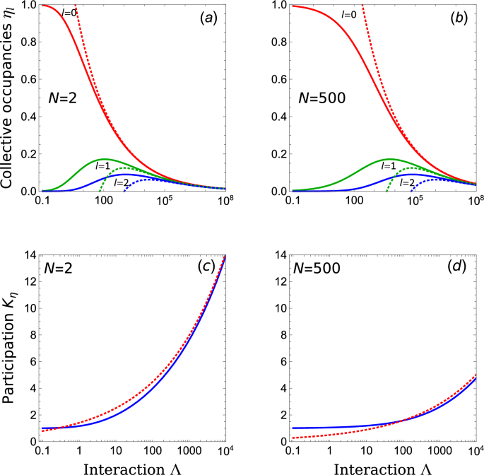
Graphs (a) and (b) show the behaviors of collective occupancies as functions of interaction strength \(\Lambda\) for two different particle numbers \(N=2\) and \(N=500\), respectively. The dashed lines represent the approximation results (30). The strength of the interaction \(\Lambda\) is expressed in units of \(m \omega ^2\). The graphs (c) and (d) illustrate the corresponding results for the participation \(K_{\eta }\), together with its approximation obtained from the expansion to infinity, \(\Lambda \rightarrow \infty\): \(K_{\eta } \approx 2\beta ^{-1}(N)\Lambda ^{1/4}\) (dashed lines).