In this section, we will introduce two quantum granular-ball generation methods: one based on iterative splitting and the other on fixed splitting numbers. To show the practicality of granular-balls, a simple application of QGBkNN is introduced.
Quantum granular-ball generation based on iterative splitting (Algorithm 1)
Quantum granular-ball generation based on iterative splitting represents the sample space by generating multiple granular-balls through iterative splitting. In the following, an example is presented to expound on the method. Consider a data points set D, each of which is characterized by a label and a 2-dimensional structure. In this instance, we assume that the dimension of the data set is 2, but it is worth noting that our algorithm can handle higher-dimensional data. The numerical values of these samples are confined to the range of \([0, 2^{h}-1]\), where h is a positive integer. Randomly extract a sample point from each data type in D as the granular-ball center, and these sample points form a granular-ball center data set \(C_0\). The remaining data points constitute the data set \(D_0\). When the i-th round of splitting ends, there will be granular-balls that meet the requirements and no longer participate in the splitting process. The remaining data points that needs to be split will form a new data set and a granular-ball center data set, reddenoted by \(D_i\) and \(C_i\), respectively. The steps for each round of iterative splitting are as follows.
The dataset \(D_i\) and the granular-ball center dataset \(C_i\) are encoded into angles. Using these angles, granular-balls are generated through a series of steps: First, the fidelity for each data point between the dataset \(D_i\) and the granular-ball center dataset \(C_i\) is calculated and is analogous to coding. Second, the analog encoded fidelity from this step is projected onto the quantum ground state. Third, the nearest granular-ball center for each data point in the dataset \(C_i\) is determined. Finally, based on the data obtained in the previous steps, new granular-balls are generated.
After the i-th round of granular-ball splitting is completed, d granular-balls are generated. The purity \(P^{i}_1\), \(P^{i}_2\), \(\ldots\), \(P^{i}_d\) of all granular-balls are computed. Based on a predefined purity threshold T, it is determined whether all granular-balls meet the requirement. No further splitting is conducted if all the purity reaches the purity threshold. Otherwise, those that fall short are extracted to the next splitting round. Among these granular-balls that need to continue to be split, randomly select heterogeneous points as the new granular-ball centers. These newly selected granular-ball centers, combined with the previous granular-ball centers in these granular-balls, form a new set of granular-ball center data \(C_{i+1}\). Simultaneously, all data points from granular-balls that can not meet the purity requirement are grouped to constitute a new data set \(D_{i+1}\). Upon the completion of data extraction and preparation, the next round of splitting is initiated. Repeat the above splitting steps till all granular-balls meet the purity requirement. The pseudocode for the quantum granular-ball generation method based on iterative splitting is shown in Algorithm 1.
Algorithm 1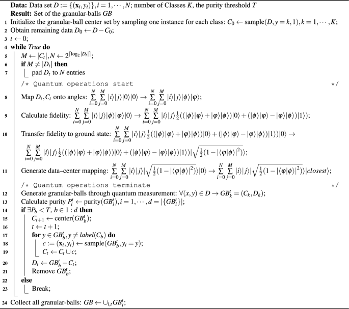
Quantum granular-ball generation based on iterative splitting
Data preparation
The initial phase of our quantum granular-ball algorithm is data preparation, which maps classical data points onto quantum states. This process involves encoding the data points of the dataset and the granular-ball center dataset as qubit angles. Let \(N_i\) represent the number of data points in dataset \(D_i\) and \(M_i\) and the number of granular-ball centers in dataset \(C_i\). Since our dataset contains two categories, we concentrate on three main issues during data encoding: data preprocessing, angle mapping, and quantum circuit preparation.
Step 1: Data preprocessing The number of data points in real-world databases is rarely a power of 2, conflicting with the quantum encoding methods that assume power-of-2 dataset sizes. To resolve this, we adjust the dataset size by padding with additional sample points to the nearest power of 2 value. For simplicity, padding data points are set to have the same values as the last data point in the dataset. Post supplementation, dataset \(D_i\) contains N data points, and dataset \(C_i\) contains M granular-ball centers.
Step 2: Angle mapping Data are then mapped to rotation angles on the Bloch sphere. Given a data value \(x=x_{h-1}\ldots x_1 x_0\) with \(x_{h-1}\) as the most significant bit, the corresponding rotation angle \(\theta _{r}\) is calculated by:
$$\begin{aligned} \theta _{r}=\pi \left( \frac{1}{2^1} \times x_{h-1}+\ldots +\frac{1}{2^{h-1}} \times x_{1}+\frac{1}{2^{h}} \times x_{0}\right) \end{aligned}$$
(10)
Note that \(\theta _{r}\) is directly proportional to x and will not exceed \(\pi\).
Step 3: Data preparation quantum circuit Both the dataset and the granular-ball center set consist of 2-dimensional points. We first introduce the data preparation for the first dimension of each dataset, followed by a combined approach for both.
The process of preparing the first dimension of the dataset into rotation angles is detailed in three stages, as depicted in Fig. 6a.
In the first stage, we use Quantum Random Access Memory (QRAM)25 to prepare data points on the ground state of the bus register, represented by the unitary operator Q. The data from dataset \(D_i\) is stored in a superposition state within \(|bus\rangle\), and this also completes the entanglement between the address register \(\vert add_D\rangle\) and the bus register \(\vert {bus}\rangle\).
The second stage employs CRY gates to encode data point from the bus register into angular qubits, with an additional angle register \(\vert ang_{D0} \rangle\) for rotation angles between 0 and \(\pi\). Using the bus register as control bits, the angles of qubit \(\vert {a}\rangle\) are encoded via CRY gates, resulting in:
$$\theta _{r} = \left( {\frac{1}{{2^{1} }} \times \left| {{\text{bus}}_{{h – 1}} } \right\rangle + \ldots + \frac{1}{{2^{{h – 1}} }} \times \left| {{\text{bus}}_{1} } \right\rangle + \frac{1}{{2^{h} }} \times \left| {{\text{bus}}_{0} } \right\rangle } \right)\pi {\text{ }}$$
(11)
The third stage reverts \(\vert {route}\rangle\) and \(\vert bus \rangle\) to their initial states using the inverse QRAM operation, allowing for the reuse of subsequent QRAM circuits.
The complete process results in the data set addresses being maintained in a superposition state within \(\vert {add_D}\rangle\), and the data values encoded in the y-axis angles of \(\vert ang_{D0} \rangle\). This entire quantum circuit is referred to as a unitary transformation \(W_D\).
Preparing the granular-ball center dataset \(C_i\) follows a similar process, as shown in Fig. 6b. This entire quantum circuit is referred to as a unitary transformation \(V_C\).
Finally, by utilizing the unitary operators \(W_D\) and \(V_C\), the preparation of all data points for both the dataset and the granular-ball center dataset is completed, as shown in Fig. 6c, and is represented as follows:
$$\left| {\psi _{a} } \right\rangle = \left| i \right\rangle _{{{\text{add}}_{D} }} \left| j \right\rangle _{{{\text{add}}_{C} }} \left| \phi \right\rangle _{{{\text{ang}}_{D} }} \left| \varphi \right\rangle _{{{\text{ang}}_{C} }}$$
(12)
where \(\left| i \right\rangle _{{{\text{add}}_{D} }}\) and \(\vert {j}\rangle _{add_C}\) are the stored addresses, and \(\vert \phi \rangle\) and \(\vert \varphi \rangle\) represent the encoded data in the angle registers \(\vert {ang_D}\rangle\) and \(\vert {ang_C}\rangle\) respectively.
Fig. 6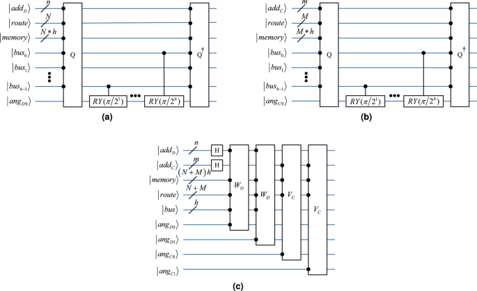
Quantum circuit for data preparation. a Preparing data points from the first dimension of the dataset, which we define as the unitary operator \(W_D\). b Preparing data points from the first dimension of the granular-ball center dataset, which we define as the unitary operator \(V_C\). c Preparing the dataset and granular-ball center dataset.
Generating new granular-balls
The generation of new granular-balls integrates concepts of fidelity calculation, fidelity transfer to the ground state, and a quantum minimum value search algorithm. The aim is to assign each data point to the nearest granular-ball center, forming new granular-balls.
Step 1: Fidelity calculation. The swap test26 Measures data-point to granular-ball center distance via fidelity between \(\vert ang_D \rangle\) and \(\vert ang_C \rangle\). Higher fidelity means closer distance.
In the quantum circuit depicted in Fig. 7, the control bit \(\vert B \rangle\) becomes a superposition state after an H gate operation.
Fig. 7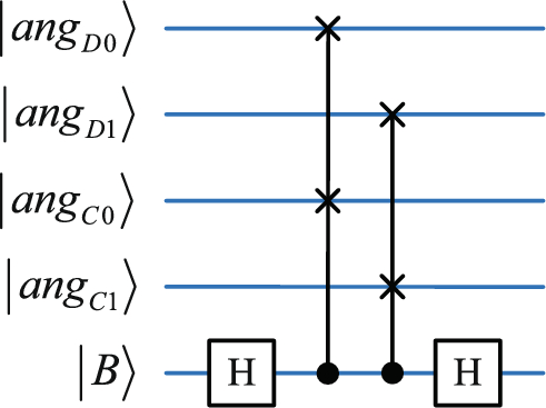
Quantum circuit for computing fidelity.
The CSWAP gates, controlled by \(\vert B \rangle\), perform SWAP operations on \(\vert ang_{D0} \rangle\) with \(\vert ang_{C0} \rangle\) and \(\vert ang_{D1} \rangle\) with \(\vert ang_{C1} \rangle\). The circuit is defined as a unitary transformation U. \(\vert \phi \rangle = \vert \phi \rangle _{ang_D}, \vert \varphi \rangle = \vert \varphi \rangle _{ang_C}\) The quantum state after the completion of the quantum circuit in Fig. 7 is as follows:
$$\begin{aligned} \begin{aligned}&\vert \psi \rangle = \frac{1}{2} ( \left( \vert \phi \rangle \vert \varphi \rangle + \vert \varphi \rangle \vert \phi \rangle \right) \vert 0 \rangle _B + \left( \vert \phi \rangle \vert \varphi \rangle – \vert \varphi \rangle \vert \phi \rangle \right) \vert 1 \rangle _B ) \\ \end{aligned} \end{aligned}$$
(13)
The relationship between \(\theta\) and fidelity is defined as \(\cos (\pi \theta ) = \sqrt{\frac{1}{2}(1 – |\langle \varphi \vert \phi \rangle |^2)}\), with \(\theta\) ranging from \(\frac{1}{4}\) to \(\frac{1}{2}\). The simplified quantum state \(\vert \psi \rangle\) is as follows:
$$\begin{aligned} \begin{aligned}&\vert {\psi _{\pm }}\rangle =\frac{1}{2}(\frac{\vert {\phi }\rangle \vert {\varphi }\rangle +\vert {\varphi }\rangle \vert {\phi }\rangle )\vert {0}\rangle _B}{\sqrt{1+{|\langle {\varphi } \vert {\phi } \rangle |}^2}}\pm \frac{\vert {\phi }\rangle \vert {\varphi }\rangle -\vert {\varphi }\rangle \vert {\phi }\rangle )\vert {1}\rangle _B}{\sqrt{1-{|\langle {\varphi } \vert {\phi } \rangle |}^2}})\\&\vert \psi \rangle = \frac{-i}{\sqrt{2}} \left( e^{i\pi \theta } \vert \psi _+ \rangle – e^{-i\pi \theta } \vert \psi _- \rangle \right) \\ \end{aligned} \end{aligned}$$
(14)
A larger value of \(\theta\) results in a smaller \(\cos (\pi \theta )\), corresponding to higher fidelity and closer proximity to granular-ball centers. Fidelity can be determined through quantum measurements on the registers, aiding in identifying the nearest center for each data point. However, this process is resource-intensive. To mitigate this, fidelity information is transferred to the ground state, which requires minimal quantum measurements for information retrieval.
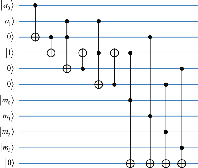
Step 2: Fidelity transfer to the ground state. Using the absolute-quantum analog to digital conversion (abs-QADC) algorithm27 to convert the angle \(\theta\) from analog to digital encoding, we first need to construct the unitary operator G. This operator G is constructed using the quantum circuit for data preparation and fidelity calculation as depicted in Fig. 8a. Once constructed, the unitary operator is \(G=UVWSW^{\dagger }V^{\dagger }\) ,as shown in Fig. 8b.
Fig. 8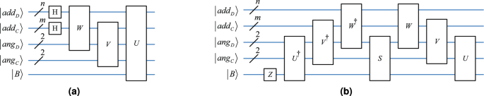
Quantum circuit for constructing the unitary operator G. a W preps the data set, V preps granular-ball center data, U calculates fidelity. b The circuit includes the inverse operations \(U^\dagger\) for U, \(V^\dagger\) for V, and \(W^\dagger\) for W. Additionally, the function of Z is to rotate \(180^{\circ }\) around the z-axis of qubit \(\vert {B}\rangle\).
As shown in the red box in Fig. 9, a t-qubit \(\vert dig \rangle\) register is added and initialized to 0 to store the digitally encoded \(\theta\). Utilizing the quantum state \(\vert \psi \rangle\), the register \(\vert dig \rangle\), and the unitary operator G, the abs-QADC quantum circuit is designed. The quantum output state of the circuit is as follows:
$$\begin{aligned} \vert { \psi }\rangle \vert {0}\rangle _t \xrightarrow {QADC} \vert {i}\rangle \vert {j}\rangle \frac{-i}{\sqrt{2}}(e^{i\pi \theta }\vert {\theta }\rangle \vert {\psi _+}\rangle -e^{-i\pi \theta }\vert {1-\theta }\rangle \vert {\psi _-}\rangle ) \end{aligned}$$
(15)
Next, we utilize the quantum cosine function algorithm28 to compute \(\cos (\pi \theta )\) with the \(\theta\) from equation 15. As shown in Fig. 9, an additional register \(\vert fidelity \rangle\) of r qubits is introduced to store the computation result \(\cos (\pi \theta )\). Using the quantum circuit COS of the quantum cosine function algorithm, the result obtained is \(\vert {i}\rangle _{add_D} \vert {j}\rangle _{add_C} \vert \cos (\pi \theta )\rangle _{fidelity}\), where \(\vert i\rangle _{add_D}\) and \(\vert j\rangle _{add_C}\) represent the addresses of the data set and the granular-ball center data set, respectively, and \(\vert \cos (\pi \theta )\rangle _{fidelity}\) indicates the digitally encoded form of \(\cos (\pi \theta )\).
Fig. 9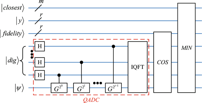
Quantum circuit for obtaining the digitally encoded \(cos(\pi \theta )\) and finding the nearest granular-ball center for each data point.
Step 3: Generate new granular-balls. By identifying the minimum \(\cos (\pi \theta )\) entangled with i, we can determine the nearest quantum granular-ball center for each data point, thereby achieving the generation of granular-balls. We have adopted the quantum minimum value search algorithm proposed in reference31 to design the corresponding quantum circuit, as shown in Fig. 9. We’ve added two new registers: the \(\vert y \rangle\), storing the initial threshold for the quantum minimum search, set to 0. The MIN in Fig. 9 represents the quantum minimum value search algorithm itself, ensuring that whenever the value in the \(\vert y \rangle\) register is updated, the address from the \(\vert add_D \rangle\) register, entangled with \(\vert y \rangle\), is copied to the \(\vert closest \rangle\) register. Another register, \(\vert closest \rangle\), stores the addresses of the nearest granular-ball centers with m qubits. After completing the quantum circuit, the final state is as follows:
$$\begin{aligned} \vert out \rangle =\vert i \rangle _{add_D} \vert closest_j \rangle _{closest} \end{aligned}$$
(16)
where \(\vert {i}\rangle _{add_D}\) represents the address i of the data set stored in a superposition state within the address register \(\vert add_D \rangle\); \(\vert {closest_j}\rangle _{closest}\) represents the address \(closest_j\) of the nearest granular-ball centers for each data point i. In this way, each data point in the data set \(D_i\) successfully finds its nearest granular-ball center.
Once all data points have found their nearest granular-ball centers, these centers and their corresponding data points can be grouped to form new granular-balls, completing one round of granular-ball generation. Subsequently, in classical computation, the purity of each granular-ball is calculated and compared with a preset purity threshold. Data points that do not meet the purity requirements will enter the next round of the loop until all granular-balls satisfy the purity requirements, thus completing the generation of all granular-balls.
Quantum granular-ball generation based on fixed splitting number (Algorithm 2)
The iterative splitting method can generate granular-balls that are suitable for the sample distribution and offer advantages in time complexity compared to classical methods. However, the hybrid model of quantum and classical and the multiple iterations required during the granular-ball splitting process lead to significant consumption of quantum resources. To overcome this issue, a new quantum granular-ball generation method based on a fixed number of splits is proposed in this paper, which can generate a fixed number of granular-balls for the entire sample space in a single operation. Moreover, it is a fully quantized process after data preprocessing. For N samples, the number of clusters produced by clustering is less than \(c_{max}\). A rule of thumb that many investigators use is \(c_{max} \le \sqrt{N}\)32,33. Reference34 has verified the correctness of this rule. We have integrated the concept of this rule to determine the number of splits to be \(\sqrt{N}\), ultimately resulting in \(\sqrt{N}\) granular-balls. Implementing the quantum granular-ball generation method that uses a fixed number of splits follows the same process as a single splitting round in the iterative splitting method.
Each of these quantum granular-ball generation methods has its own set of strengths and weaknesses. Algorithm 1 is notable for its ability to generate granular-balls that are well-adapted to the data distribution, which is a significant advantage, but it also requires multiple iterations and conditional judgments, potentially leading to a more complex process.
Algorithm 2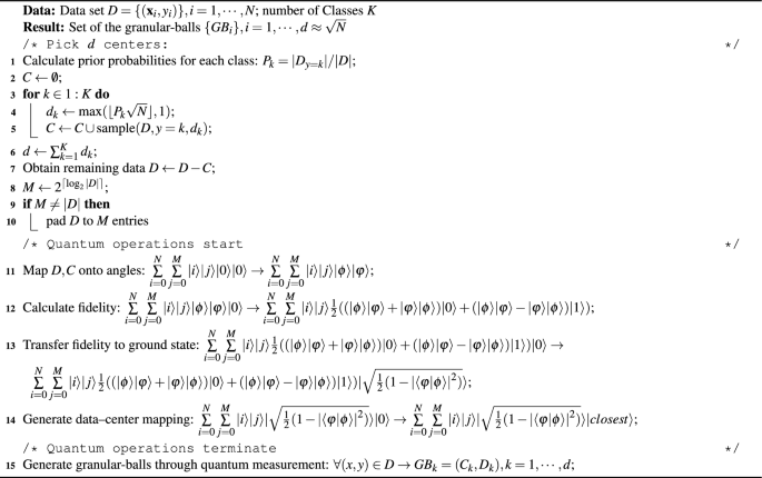
Quantum granular-ball generation by fixed splitting
In contrast, Algorithm 2, due to its fixed number of splits, is capable of rapidly and simultaneously splitting all granular-balls. It can achieve full quantization without the need for multiple switches between classical and quantum computations. However, the downside is that it may produce an inappropriate number of granular-balls, The pseudocode for the quantum granular-ball generation method based on a fixed splitting number is shown in Algorithm 2.
Quantum k-nearest neighbors algorithm based on granular-balls
The current QkNN enhances efficiency by leveraging quantum entanglement and quantum parallelism. However, the efficiency of both kNN and QkNN is constrained by large-scale data sets. To address this issue, this paper uses granular-balls to represent large data sets for implementing the kNN. The core concept of QGBkNN is to apply the quantum granular-ball generation method to the training set, using granular-balls to represent the entire sample space, allowing test samples with unknown labels to determine their category based on the category of the nearest granular-ball center. Since each granular-ball represents multiple samples with the same label from the training set, it is sufficient to set k to 1. The algorithm consists of two stages:
-
(1)
Training: generate the quantum granular-balls, and replace the original training set with the generated granular-balls.
-
(2)
Testing: Assign the test sample’s category based on its nearest granular-ball center.
Suppose a training set of N samples and a test sample. The dimensions of the training set and the sample dimensions of the test sample points are both 2, and the value range is \([0, 2^h-1]\). Taking the training set and test sample as examples, the two steps of QGBkNN are analyzed as follows.
The first step involves converting the sample points in the training set into granular-balls and using the granular-ball centers as the new training set E. The number of granular-balls generated by the quantum granular-ball generation method based on iterative splitting is uncertain, while quantum granular-ball generation based on a fixed splitting number generates \(\sqrt{N}\) granular-balls. The second step involves determining the test sample determining its category based on the nearest granular-ball center. This process is similar to the concept of finding the nearest granular-ball center and includes the following steps: first, encoding the training set E and the test sample point into angles; then, calculating the fidelity between the test sample point c and the training set E; transferring the analog encoded fidelity to the ground state; and finally, identifying the most similar sample point to the test sample point within the training set. It is worth noting that the QGBkNN based on Algorithm 2 needs to add another step to further increase its classification accuracy, which is that after the measurement, the label of the majority of the selected granular-ball is taken as the label of the test sample point. The pseudocode for the Quantum k-nearest neighbors algorithm based on granular-balls is shown in Algorithm 3.
Algorithm 3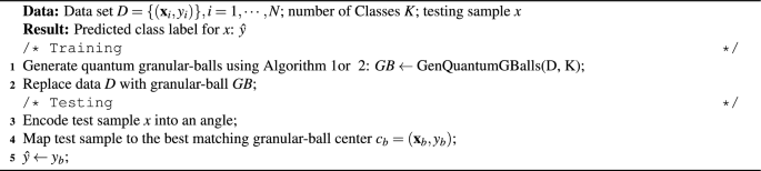
Quantum granular-ball nearest neighbour classification
Performance analysis
This subsection aims to conduct a comparative analysis of the time complexity between the two quantum granular-ball generation methods developed and their corresponding classical counterparts. Subsequently, a performance comparison will be made between the proposed QGBkNN algorithm and other kNN algorithms.
To make the explanation clearer, we provide the following clarification. The time complexity we evaluate is the depth of the quantum circuit of the quantum algorithm, and both the quantum circuit depth of the algorithm and the time complexity assessment are related to the steps of the algorithm’s execution. Therefore, we directly equate the quantum circuit depth of the algorithm with its time complexity for description to achieve uniformity and facilitate performance comparison with subsequent algorithms.
Time complexity analysis of quantum granular-ball generation methods
Time complexity analysis of Algorithm 1: During one splitting round, the data preparation time complexity is \(O(\log {MN})\), where M is the number of granular-balls and N is the number of samples. The time complexity of the abs-QADC is related to the number of bits to be estimated, and it is \(O((\log ^{2}{MN})/2^{-t})\). Due to the limited number of estimated bits, we simplify it to \(O(\log ^{2}{MN})\). The time complexity of the quantum cosine function quantum circuit is not dependent on the data set or dimensionality, so it is O(1). The time complexity of finding the nearest granular-ball center is \(O(\sqrt{M}\log ^{2}{MN})\). The overall time complexity for one round of splitting is \(O(\log {MN}+\log ^{2}{MN}+(\log ^{2}{MN})\sqrt{M})=O(\sqrt{M}\log ^{2}{MN})\). Assuming a total of d iterations, the total time complexity is \(O(d(\log ^{2}{MN})\sqrt{M})\).
Time complexity analysis of Algorithm 2: The number of data points is N, and the number of granular-ball center data points is \(\sqrt{N}\). The data preparation time complexity is \(O(\log {N^{\frac{3}{2}}})=O(\log N)\). The time complexity for fidelity transfer to the ground state is \(O(\log ^{2}{N})\). The time complexity for finding the nearest granular-ball center is \(O((\log ^{2}{N})N^\frac{1}{4})\). The overall time complexity is \(O(\log {N}+\log ^{2}{N}+(\log ^{2}{N})N^\frac{1}{4})=O((\log ^{2}{N})N^\frac{1}{4})\).
Table 1 compares the time complexity of two quantum granular-ball generation algorithms with that of the classical granular-ball generation algorithm. Currently, the time complexity of the classical granular-ball generation algorithm is O(mdN), where m is the number of granular-balls. Algorithm 1 reduces the time complexity to \(O(\sqrt{M}\log ^{2}{MN})\), with M being the number of data points in the granular-ball center dataset, which is significantly less than N. Algorithm 2 further eliminates the iterative process, thereby reducing the time complexity to \(O((\log ^{2}{N})N^\frac{1}{4})\).
Table 1 Comparisons of the time complexity of quantum granular-ball generation methods.Comparison of performance between QGBkNN and other kNN algorithms
Regarding time complexity, as shown in Tab. 2, QGBkNN proposed in this paper reduces the time complexity compared to GBkNN13, and QkNN.
Table 2 Performance analysis of quantum kNN variants.