We simulated rock extraction under three rock supply scenarios, each with different production targets by 2070: S1, low rock supply (32 Mt yr−1), S2, medium rock supply (97 Mt yr−1) and S3, high rock supply (166 Mt yr−1). These scenarios, which are consistent with scenarios defined in previous studies18, necessitate substantial upscaling. This upscaling is modelled as an annual growth rate applied to the existing capacity of individual quarries until their production reaches a specified maximum annual cap. Our initial analysis assessed the impact of varying annual growth rates and production caps on the upscaling pathways and resulting CDR. Historical data on crushed rock production from 196018 to the present reveal that annual growth rates can vary widely, reaching up to 50%. These fluctuations are driven by variable supply and demand, but are not necessarily indicative of the potential rate; the largest 10-year rolling average of 15% may be a more suitable indicator of potential rate. Consequently, we constrained scenarios with a base-case of 15% but examined the model sensitivity of growth rates ranging from 5 to 50%, and considered three annual production caps of 1, 2 and 5 Mt yr−1 for individual quarries. A summary of the scenarios simulated in this study, along with their features, is presented in Table 1.
Table 1 Summary of scenario codes, descriptive names and key differentiating features: target supply by 2070 (Mt yr−1), per-quarry capacity cap (Mt yr−1) and contributing quarry types
Across all scenarios with the same cumulative rock extracted (See Supplementary Information Fig. S1), more rapid annual growth rates in quarry capacity led to larger cumulative CDR. This effect is particularly substantial when growth rates increase from 5 to 15%, potentially resulting in up to 15% more CDR. Similarly, increasing the annual production cap from 2 to 5 Mt yr−1 per quarry led to an additional 13% in CDR by 2070. Lifting constraints on growth rates and production caps enables the model to prioritise quarries with more favourable conditions, allowing them to contribute more substantially and earlier to the rock supply, thereby enhancing CDR efficiency.
Our models showed that relying only on the expansion of existing active quarries for fulfilling the target demand requires over 30 mega-quarries (quarries with over 1 Mt yr−1 capacity) to operate by 2070 (Supplementary Information Fig. S2). To fulfil the target demand, the pathways were designed by following one or a combination of two or three strategies: expansion of currently active quarries, reactivating inactive quarries and opening new quarries (Supplementary Information Fig. S3).
Cumulative rock supply
Deployment scenarios have been compared by metrics including cumulative rock extracted (between 2025 and 2070), cumulative CDR, transport capacity required, average CDR rate and the number of unique quarries contributing to rock supply for all scenarios (S1, S2.a, S2.b, S3.a, S3.b and S3.c). The results are summarised in Table 2.
Table 2 Cumulative metrics (for the years ranging 2025–2070) including cumulative rock extracted, cumulative CDR, transport capacity required, average CDR rate and the number of unique quarries contributing to rock supply for all scenarios (S1, S2.a, S2.b, S3.a, S3.b and S3.c)
In Scenario S1 (low rock supply), a cumulative total of 1.1 Gt of rock is extracted, reflecting a conservative approach focused on expanding currently active quarries. This results in a cumulative CDR of 175 Mt CO2. In Scenarios S2.a (Medium rock supply, active only) and S2.b (Medium rock supply, active and inactive), the cumulative rock extracted is substantially greater, at 2.4 Gt, driven by moderate upscaling efforts. Scenario S2.a achieves a cumulative CDR of 348 Mt CO2 by 2070, due to higher production caps at active quarries. In contrast, Scenario S2.b, which includes reactivating inactive quarries, achieves a slightly lower cumulative CDR of 336 Mt CO2 by 2070 due to the limited production cap of 1 Mt yr−1. Please note that the efficiency drop from S2.a to S2.b is not inherently due to adding inactive quarries. Higher production caps (e.g. 2 Mt yr−1) give the model more freedom to allocate production to the most favourable sites, whereas a tighter 1 Mt yr−1 cap spreads production across a wider, and generally less optimal, pool of quarries.
The high rock supply scenarios (S3.a,b,c) involve the larger extraction of 4.7 Gt of rock, reflecting a substantial upscaling effort. Scenario S3.a (High rock supply, active only) achieves a cumulative CDR of 703 Mt CO2, demonstrating the efficiency of concentrating rock extraction in a smaller number of high-capacity quarries (47 mega quarries). Scenario S3.c, (High rock supply, active, inactive and new), on the other hand, achieves a lower cumulative CDR of 58 Mt CO2 and faces higher logistical demands (1975 t.km tCO2−1) compared to S3.a (1227 t.km tCO2−1). Scenario S3.b (High rock supply, active and inactive), which combines the expansion of active quarries with the reactivation of inactive quarries, achieves a cumulative CDR of 639 Mt CO2, indicating the benefits of a balanced approach.
The mean CDR rate (t CO₂ per t rock) declines as supply targets increase, illustrating a clear scale-efficiency trade-off. Because the model always allocates rock first to the highest CDR yield quarry-cropland pairs, average CDR rate (efficiency) inevitably falls as supply targets rise: once the allocations of most favourable quarry-cropland pairs have been fulfilled, meeting the larger medium and high supply targets (S2 and S3) requires the model to draw on progressively less favourable combinations. Lower per‑quarry annual production caps accentuate this effect by spreading production across more, and often less favourable quarries, whereas higher caps (e.g. 2 and 5 Mt yr−1 in S2.a and S3.a, respectively) let extraction concentrate at the most efficient sites and partly offset the decline.
Rock transport required per tonne of CO2 removed from the atmosphere has direct implications for the CDR efficiency. Scenario S2.a (Medium rock supply, active only) demonstrates the lowest transport requirements among all scenarios, while S3.a (High rock supply, active only) shows the best efficiency among the high supply scenarios. The average CDR rate provides insight into the effectiveness of CO2 removal per unit mass of rock used and has implications for the CDR cost associated with rock extraction, grinding, transport and spreading, with scenario S1 (low rock supply) and S3.c (High rock supply, active, inactive and new) having the highest and lowest rate respectively.
Temporal evolution of rock supply
Target rock demand scenarios along with corresponding temporal evolution of key metrics, including CDR, transport capacity required and CDR rate for all scenarios is presented in Fig. 1.
Fig. 1: Potential of enhanced rock weathering in the UK 2025–2070.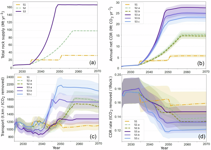
a Target annual rock supply scenarios from Kantzas et al. (2022), b corresponding annual net carbon dioxide removal, c transport requirements, and mean CDR d efficiency per tonne of rock. Description of scenarios: S1, Low rock supply scenario, cap 1 Mt yr−1. S2.a, Medium rock supply scenario, cap 2 Mt yr−1. S2.b, Medium rock supply scenario, cap 1 Mt yr−1. S3.a, High rock supply scenario, cap 5 Mt yr−1. S3.b, High rock supply scenario, cap 2 Mt yr−1. S3.c, High rock supply scenario, cap 1 Mt yr−1. Shaded envelopes represent the uncertainty arising from variation in rock max CDR potential. (see Supplementary Data 1).
The annual CDR, depicted in Fig. 1.b, shows an increasing trend across all scenarios over time consistent with the rock supply. By 2070, the CDR can range from 6 to 27 Mt yr−1 of CO2, depending on the scenario chosen. Despite having the same amount of rock supplied, the CDR achieved varies substantially between sub-scenarios within S3 (High rock supply). For instance, Scenario S3.a (High rock supply, active only) shows (~20%) higher CDR compared to S3.c (High rock supply, active, inactive and new), and a more pronounced difference (~35%) in transport requirement. However, prior to 2045, these differences in CDR between sub-scenarios are minimal due to the rapid expansion required, necessitating the utilisation of all available resources and leaving little room for optimisation. But, after 2050, as demand stabilises and quarry capacities have expanded, the model can better optimise resource allocation, resulting in substantial variations in CDR among different sub-scenarios. By 2070, the S3.a (High rock supply, active only) captures up to 5 Mt yr−1 more CO2 than S3.c (High rock supply, active, inactive and new), highlighting the effectiveness of optimised resource allocation.
From 2025 to 2035, the transport requirements decrease while the CDR rate increases. This period reflects the model’s ability to prioritise effectively under relatively low demand. However, between 2035 and 2050, the trend reverses: transport requirements increase, and CDR rates decrease due to the need to supply croplands at greater distances and the rapid surge in demand, which limits the model’s optimisation potential. Post-2050, as demand stabilises, the trend improves again and the difference in efficiency between sub-scenarios (especially within high rock supply scenarios, S3) becomes more pronounced, showcasing the enhanced optimisation potential under stable demand and up-scaled rock supply conditions.
Among high supply scenarios, Scenario S3.a (High rock supply, active only) has the most efficient logistics over time, followed closely by S3.b (High rock supply, active and inactive), while S3.c (High rock supply, active, inactive and new) faces the highest transport requirements. Post-2050, scenario S3.a exhibits a more pronounced decline in transport requirements compared to other scenarios, so that by 2070, S3.a achieves approximately 35% less transport effort per unit mass of CDR than S3.c. Scenario S3.c exhibits the lowest average CDR rate among all scenarios, whereas S3.a appears more efficient among the high rock supply scenarios. Notably, after 2055, S3.a surpasses the efficiency of even the S2 (Medium rock supply) scenarios.
Spatial distribution of rock extraction for ERW
The spatial and temporal distribution of rock extraction sites for ERW in the UK by 2070 for the largest rock supply scenario (S3) is shown in Fig. 2. The varying combination of active, inactive and new quarries results in gradual increase in the number and geographic reach of quarries by moving from scenario S3.a (High rock supply, active only) to S3.b (High rock supply, active and inactive) and S3.c (High rock supply, active, inactive and new), leading to a broader distribution across the UK in S3.c. However, the overall pattern remains uneven, with extraction sites predominantly concentrated in the central belt of Scotland and Northern Ireland (NI).
Fig. 2: Spatial and temporal distribution of quarries and their annual production capacity.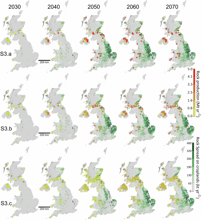
Maps show annual rock production from quarries and the quantity of rock spread on croplands (10 × 10 km grid cells) across the UK for years 2030, 2040, 2050, 2060 and 2070 under three sub-scenarios: S3.a (top row), S3.b (middle row) and S3.c (bottom row). The background grid represents rock application on cropland, shaded from white to dark green, where darker shades indicate greater quantities of rock spread per grid cell.
In Scenario S3.a, which relies solely on the expansion of currently active quarries, rock supply is met by a smaller number of quarries, with gradual increases in their production capacity and high-capacity quarries (up to 5 Mt yr−1) emerging from 2050. Notably, in 2040, the number of contributing quarries in NI temporarily decreases, highlighting the model’s preference for utilising a minimum number of more favourable quarries.
Scenario S3.b involves a reactivation of inactive quarries from 2040, with a combination of existing and reactivated quarries contributing to production toward 2070. Several quarries are reactivated around the Midlands and North-East England with close proximity to abundant croplands.
From 2050 and continuing to 2070 in Scenario S3.c, new quarries begin operations and contribute to the rock supply alongside reactivated and existing quarries. Due to the maximum cap for each individual quarry being limited to 1 Mt yr−1, reactivated quarries, such as those in NI, start contributing to the rock supply as early as 2040 to ensure fulfilling the target demand. The distribution of new quarries is concentrated mainly in the Central Belt of Scotland, NI, Northern Wales, South-West and North-East England and the North West of Scotland.
The background map in Fig. 2 shows the cropland grid cells and the amount of rock spread onto cropland in each grid cell. While croplands nearer to quarries receive rock in the early years, most of the supplied rock is ultimately applied to the central and eastern regions of England. This is because these regions have more extensive areas of cropland. Additionally, a substantial portion of the rock supply from NI reaches these regions via the Felixstowe port, owing to its proximity to high-efficiency croplands and convenient transport logistics. See Supplementary Information Fig. S4 for the locations of the main ports and the shipping routes contributing to the supply of rock from NI to Great Britain (GB) for ERW.
In addition to spatial distribution, the temporal prioritisation in the model has led to varying contributions from active, inactive and new quarries to the total rock supply for ERW over time, as shown in Fig. 3. In Scenarios S3.b (High rock supply, active and inactive) and S3.c (High rock supply, active, inactive and new), the contribution to the total rock supply exhibit substantial shifts over the years. Initially, active quarries dominate the supply, but as time progresses, reactivated and new quarries increasingly contribute, especially post-2045. In scenario S3.c, by 2070, new quarries form a substantial part of the supply chain, highlighting the model’s strategy to open new extraction sites to meet the increasing demand. After 2050, as the demand stabilises, existing quarries have had sufficient time to expand their production capacity. Consequently, the model allocates more rock to expanded existing quarries, leading to a slight decline in the contribution from new and reactivated quarries toward 2070.
Fig. 3: Normalised contribution of active, reactivated and new quarries to the rock supply for ERW in the UK.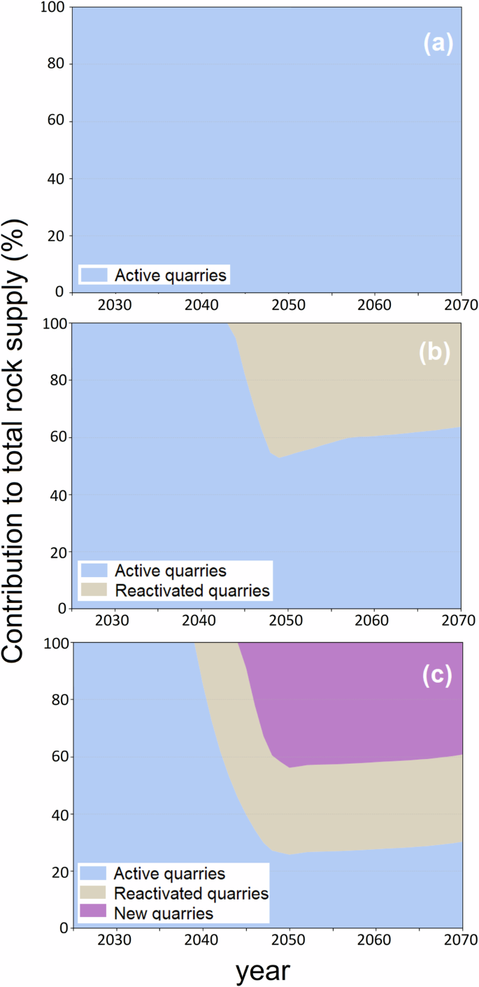
a Scenario S3.a, (High rock supply, active only), b Scenario S3.b, (High rock supply, active and inactive) and c Scenario S3.c (High rock supply, active, inactive and new). (see Supplementary Data 2).
Resource requirements, flow and logistics
The analysis of rock supply requirements by counties and countries for ERW in the UK reveals substantial regional variation in the demands and reserves needed by 2070. Fig. 4 illustrates these differences across the three largest rock supply scenarios (S3.a, S3.b and S3.c).
Fig. 4: Annual rock extraction in 2070, cumulative reserve requirements and Extraction density across UK counties under S3 sub-scenarios.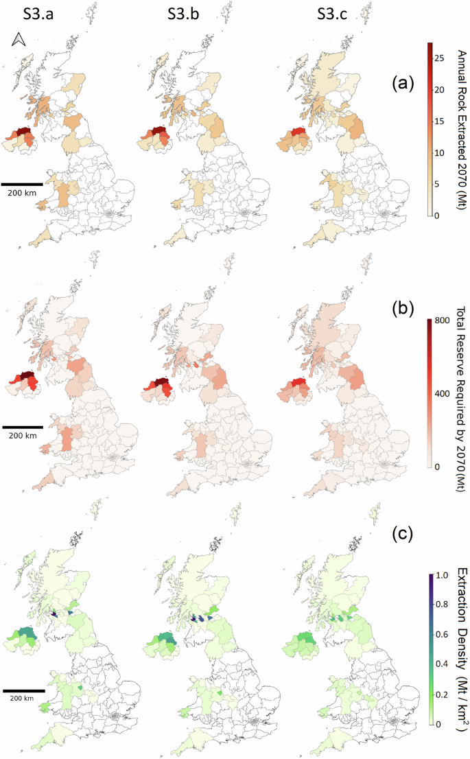
a Annual rock production by county in year 2070 b cumulative reserve required by 2070 by county in different S3 (High rock supply) sub-scenarios. c Extraction density as a metric representing the cumulative reserve requirement divided by the county area, illustrating the potential concentrated environmental and social impact of extraction activities in each county.
In 2070, Scenario S3.a (High rock supply, active only) shows a substantial concentration of rock extraction activities in smaller number of counties, with capacities exceeding 25 Mt yr−1 in some jurisdictions. Scenario S3.b (High rock supply, active and inactive) introduces notable contributions from North Scotland, Midlands and North East England in addition to the contributing counties in S3.a. Scenario S3.c (High rock supply, active, inactive and new), with its lowest production cap per individual quarry (1 Mt yr−1), results in a more widespread but less intensive distribution of extraction activities across counties.
The total reserve requirement by 2070 also highlights these regional differences. In S3.a (High rock supply, active only) and S3.b (High rock supply, active and inactive), NI and the Central Belt of Scotland require substantial reserves, up to 800 Mt in some counties. Scenario S3.c (High rock supply, active, inactive and new) distributes the reserve requirements more evenly across the UK, though NI and Scotland still dominate.
The concentration of rock extraction activities within a specific area is illustrated by county in Fig. 4 (bottom row). The data reveal a high concentration of extraction activities in NI (particularly Northern Antrim and Derry/Londonderry) and the Central Belt of Scotland (Renfrewshire, North Lanarkshire, Edinburgh). Progressing from Scenario S3.a (High rock supply, active only) to S3.b (High rock supply, active and inactive) and S3.c (High rock supply, active, inactive and new), the intensity of these extraction activities is distributed more evenly across additional counties, reducing the concentration in any single county and thus potentially reducing the localised environmental and social impacts.
County‐based extraction density maps can distort the true burden of quarrying activities because counties vary widely in size: high extraction in a large county may appear as a low extraction density, while the same extraction in a small county yields a much higher extraction density. This area dependence can obscure real intensity peaks. However, county boundaries correspond to local‐authority administrative regions responsible for planning permissions and community impacts, making county-scale density maps directly applicable for policymakers. For a more consistent spatial view, we also computed extraction density on a uniform 10 × 10 km grid (Fig. S6 in Supplementary Information). While these grid-based patterns generally align with the county-level results, they more clearly show how higher per-quarry production caps (S3.a) concentrate high-density extraction into a few hotspots, whereas more constrained production caps (S3.b and S3.c) diffuse this burden more evenly across the UK.
The contribution of the UK’s countries to rock extraction and spreading on croplands by 2070 is shown in Fig. 5a, for Scenario S3.c (High rock supply, active, inactive and new). The flow of rock supply from producing countries to croplands of different countries where the rocks will be spread for ERW is shown by flow channels with width of each flow is proportional to the quantity of rock (in million tonnes) transported.
Fig. 5: Transport requirement for ERW in the UK under the high rock supply scenario (S3.c).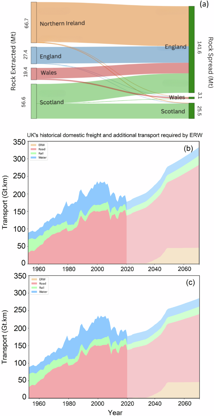
a Flow of rock supply from producing countries to croplands of different countries where the rocks will be spread for ERW. Width of each flow channel is proportional to the quantity of rock transported. And historical domestic freight transport in the UK and projected additional transport capacity required by Enhanced Weathering (ERW) by 2070, assuming 1.1% (b) and 0.7% (c) annual growth rate for baseline freight demand. These results are based on the data of transport requirement for scenario S3.c (High rock supply, active, inactive and new) as the most transport-intensive scenario. (see Supplementary Data 3).
NI and Scotland are the primary rock producers, contributing a combined total of 123.3 Mt yr−1, which accounts for over 70% of the total rock supply. England, which produces 27.4 Mt yr−1 (16% of the total rock supply), is the main region for rock application, with 141.6 Mt yr−1 being spread on its croplands by 2070, representing more than 80% of the total rock spread. NI, the largest producer with 66.7 Mt yr−1 transports all extracted tock to England and Scotland. This indicates a substantial need for dedicated transport routes.
Figure 5b, cpresents the UK’s historical domestic freight transport by mode (road, rail, water) alongside the additional capacity required for ERW rock haulage through to 2070. From 1953 to about 2000, total freight rose from roughly 90 Gt·km to a peak near 225 Gt·km, then declined to around 155 Gt·km by 2020. We project baseline freight demand under two compound‐growth projections, 1.1% p.a. and 0.7% p.a23. (NIC, 2019), shown in Fig. 5b, c, respectively. Onto each baseline we add ERW demand for the most transport‐intensive scenario (S3.c), which begins around 2025, ramps up to ~50 Gt·km yr−1 by 2045 and then plateaus. By 2050, the sum of baseline plus ERW freight demands surpasses the historic peak in both projections, reaching approximately 330 Gt·km by 2070 under 1.1% growth and 270 Gt·km under 0.7% growth.