Game theory is a mathematical method for selecting a strategy that maximizes the profits of each agent in the presence of multiple parties.27 In a game, the insteractions between players are mutual, and each player’s decision will have an impact on other players in the game. The purpose of game theory is to balance the interests of each player in each game with sufficient rationality, and achieve the maximization of the interests of each player in each game.
Mathematical model
The mathematical model of game theory mainly includes three elements: players, strategy set, and utility function, represented as \(\xi (N,I,\partial )\). N is the set of players in the game, I represents the set of players offloading pure strategies, and \(\partial\) is the utility function of the strategy combination in this situation.
(1) Bureau personnel: also known as decision-makers. An individual or group that can decide their own course of action during a game. One characteristic of game theory is that each player in the game is srational”, meaning that each player will choose their most suitable strategy based on the decisions of other players in order to maximize their own interests and there is no sense of luck (thinking that other players have made wrong decisions).
(2) Strategy set: A set of decisions in a game that players can choose from, including all the decisions made by players in a certain situation. The policy set is divided into pure policy set and mixed policy set. Given information, if only specific decisions can be selected from the policy set, it is called a pure policy set; if a certain probability is selected from the policy set, it is called a mixed policy set.
(3) Utility function: It represents the mapping relationship between a comparable value and the benefits of players in a given situation. Utility function is the fundamental basis for making decisions in game situations.
During the entire game process, player r chooses a strategy set of \(I_{r}\), where one decision in \(I_{r}\) is \(a_{r}\). Then, player r’s decision set can be represented as \(I_{r} \left( {a_{1} , \cdots ,a_{r – 1} ,a_{r} ,a_{r + 1} , \cdots ,a_{m} } \right)\) or \(\left( {a_{r} ,a_{ – r} } \right)\), where \(a_{ – r} = \left( {a_{1} , \cdots ,a_{r – 1} ,a_{r + 1} , \cdots ,a_{m} } \right)\) represents the set of decisions made by other players except for node r’s decision \(a_{r}\). Throughout the entire task execution cycle, the decisions made by each player in the game change with the changing situation, and the cost paid is represented by a utility function. Therefore, the utility function of player r in the game is \(\partial_{r} \left( {a_{r} ,a_{ – r} } \right)\) or \(\partial_{r} \left( {a_{1} , \cdots ,a_{r – 1} ,a_{r} ,a_{r + 1} , \cdots ,a_{m} } \right)\).
Optimal decision modeling
The decision space of the video stream cluster in a certain situation is K, and the mobile node \(j_{n}\) is given a policy set \(k_{{ – j_{n} }}\) in a certain state. Therefore, \(j_{n}\) can assign the optimal value to the decision variable EE based on \(k_{{ – j_{n} }}\), that is, choose the optimal decision to achieve the minimum offloading cost. The cost function can be expressed as:
$$\partial_{{j_{n} }} \left( {k_{{j_{n} }} ,k_{{ – j_{n} }} } \right) = \left\{ {\begin{array}{*{20}l} {\gamma_{{j_{n} }} T_{{j_{n} }}^{l} + \eta_{{j_{n} }} E_{{j_{n} }}^{l} ,k_{{j_{n} }} = 0} \hfill \\ {\gamma_{{j_{n} }} \left( {T_{{j_{n} ,s_{1} }}^{tran} + T_{{j_{n} ,s_{1} }} } \right) + \eta_{{j_{n} }} E_{{j_{n} ,s_{1} }}^{tran} ,k_{{j_{n} }} = 1} \hfill \\ {\gamma_{{j_{n} }} \left( {T_{{j_{n} ,s_{2} }}^{tran} + T_{{j_{n} ,s_{2} }} } \right) + \eta_{{j_{n} }} E_{{j_{n} ,s_{2} }}^{tran} ,k_{{j_{n} }} = 2} \hfill \\ \end{array} } \right.$$
(25)
The cost of uninstalling a node can be expressed as:
$$\partial_{{j_{n} }} \left( {k_{{j_{n} }} } \right) = \min \partial_{{j_{n} }} \left( {k_{{j_{n} }} ,k_{{ – j_{n} }} } \right)$$
(26)
where, \(T_{{j_{n} }}^{sum \, } \le T_{{j_{n} }}^{\max }\) indicates that the processing time per unit task cannot exceed the maximum delay \(T_{{j_{n} }}^{\max }\), and the value of \(k_{{j_{n} }}\) is the optimal decision for \(j_{n}\) in this situation.
Principle of task offloading
The ultimate outcome of the game is to reach Nash equilibrium, which is defined as follows.
Definition 1
(Nash equilibrium) In a game \(\xi = \left\{ {I_{1} , \cdots ,I_{N} ;\partial_{1} , \cdots ,\partial_{N} } \right\}\) involving N players, the optimal decision is made for any player whose decision \(i_{ – r}^{*} = \left( {i_{1}^{*} , \cdots ,i_{r – 1}^{*} ,i_{r + 1}^{*} , \cdots ,i_{N}^{*} } \right)\) in other games is the best. If:
$$\partial_{r} \left( {i_{r}^{*} ,i_{ – r}^{*} } \right) \le \partial_{r} \left( {i_{r} ,i_{ – r}^{*} } \right)$$
(27)
Then \(\partial_{r} \left( {i_{r}^{*} ,i_{ – r}^{*} } \right)\) is called a Nash equilibrium in the game.
Taking a certain state (i.e. the position and offloading decision of all video streams in each time slot) as a situation, the set of players N in the game consists of n video streams, the set of strategies made by each player in a certain state is, and the set of decision costs adopted in this state is \(\partial\). The basic model \(\xi \left( {N,I,\partial } \right)\) of the game can be obtained from the players, the set of strategies, and the cost function. The offloading model time slot diagram is shown in Fig. 2. In a certain time slot \(\Delta t\), there exists a time t that satisfies \(t \in \Delta t\). When the time slot \(\Delta t\) is small enough, the cluster video stream reaches a stationary state. At time t, the video stream \(j_{n}\) estimates the offloading cost to determine whether the current decision is optimal. If it is not the optimal decision, the offloading update is executed. In time slot \(\Delta t\), all video streams loop through this process until the decision for each video stream is optimal.
Fig. 2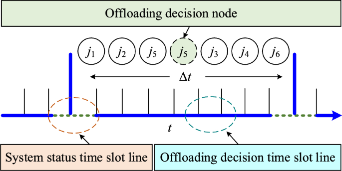
Time slot diagram of offloading model.
Theorem 1
In the game process, for i, \(\forall i_{r} \in I_{r}\), \(\forall r \in N\), and I as the strategy set, if \(\partial_{r} \left( {i_{r}^{*} ,i_{ – r}^{*} } \right) \le \partial_{r} \left( {i_{r} ,i_{ – r}^{{}} } \right)\) satisfies \(\phi \left( {i_{r}^{*} ,i_{ – r}^{*} } \right) \le \phi \left( {i_{r} ,i_{ – r}^{*} } \right)\), then this game is called a potential game. Moreover, there exists at least one Nash equilibrium in a potential game that satisfies:
$$\phi \left( {k_{j}^{*} ,k_{ – j}^{*} } \right) – \phi \left( {k_{j} ,k_{ – j}^{*} } \right)\partial = \partial_{j} \left( {k_{j}^{*} ,k_{ – j}^{*} } \right) – \partial_{j} \left( {k_{j} ,k_{ – j}^{*} } \right)$$
(28)
where, \(\phi \left( {k_{j}^{*} ,k_{ – j}^{*} } \right) = \min \partial_{j} \left( {k_{j} ,k_{ – j} } \right) = \varphi \left( {k_{j}^{*} } \right)\) and \(\varphi \left( {k_{j}^{*} } \right)\) are the minimum values of the price when node j makes the optimal decision k, \(k \in \left\{ {0,1,2} \right\}\), \(j \in N\). Therefore, for the cost function \(\partial_{j} \left( {k_{j} ,k_{ – j} } \right)\) of the multi video stream offloading game model, satisfying the potential function equation \(\phi \left( {k_{j}^{*} ,k_{ – j}^{*} } \right) \le \phi \left( {k_{j} ,k_{ – j}^{*} } \right)\) is a potential game.
Proof
Define mapping \(\phi :K \to K\), where \(\phi \left( k \right) = \left( {\phi_{1} \left( {k_{ – 1} } \right), \cdots ,\phi_{n} \left( {k_{ – n} } \right),\phi_{i} \left( {k_{ – i} } \right)} \right)\) represents the optimal response strategy of participant k to other participant strategies \(k_{ – i}\), i.e. \(\phi_{i} \left( {k_{ – i} } \right) \in \arg \max U_{i} \left( {k_{i}^{ * } ,k_{ – i} } \right)\). Due to the continuity of the utility function \(\partial_{i} \left( k \right)\), the optimal response \(\phi_{i} \left( {k_{ – i} } \right)\) is also continuous. The strategy space \(S\) is a non empty compact convex set, and the optimal response mapping maintains a convex combination (if \(k,k^{ * } \in S\), then \(\lambda k + \left( {1 – \lambda } \right)k^{ * } \in K\)).
According to Brouwer’s fixed point theorem, the continuous mapping \(\phi\) has at least one fixed point \(k^{ * }\), i.e. \(\phi \left( {k^{ * } } \right) = k^{ * }\), on the convex compact set \(S\). At this point, \(k^{ * }\) is a Nash equilibrium, as any participant cannot increase returns by unilaterally changing their strategy.
Therefore, considering a multi video stream offloading game model, the cost function \(\partial_{j} \left( k \right)\) satisfies the potential function equation:
$$\phi \left( {k_{j}^{*} ,k_{ – j}^{*} } \right) – \phi \left( {k_{j} ,k_{ – j}^{*} } \right) = \partial_{j} \left( {k_{j}^{*} ,k_{ – j}^{*} } \right) – \partial_{j} \left( {k_{j} ,k_{ – j}^{*} } \right)$$
where, \(k\) represents the uninstallation strategy, and \(\phi \left( k \right)\) is the overall situation function. Due to the continuity of the potential function \(\phi \left( k \right)\) and the compactness of the strategy space S, according to the potential game theory, there exists at least one pure strategy Nash equilibrium theorem. Therefore, the multi video stream offloading game model has at least one pure strategy Nash equilibrium. Certificate completed.
In the decision-making process of unloading multiple data streams, in order to ensure that the system can efficiently and reasonably handle all kinds of video streams, we do not simply prioritize the streams. Based on the optimization model shown in formula (10), we adjust the delay weight. For video streams with high real-time requirements, we set a larger weight value \(\phi\), and its energy consumption index weight value 1-\(\phi\) will be reduced accordingly, so as to tilt its delay index. For example, the real-time monitoring video stream has high requirements for low delay, because any delay may lead to the omission of key information; The VOD stream has a slightly higher tolerance for delay, but has higher requirements for video quality and playback fluency. In this scenario, there exists a Nash equilibrium in a finite game (limited strategy space) and it is unique, meaning that every decision to unload a video stream is the best option, achieving a Nash equilibrium.
Node \(j_{n}\) is a mobile node, also known as \(j_{n} \in N\). The decision space during the entire task execution process is K, and every time \(T_{{{\text{slot}}}}\), the video stream executes the offloading and updating algorithm in a certain state. Node \(j_{n}\) estimates the cost of executing the task. If the decision \(k_{{j_{n} }}\) satisfies:
$$\partial_{{j_{n} }}^{t} \left( {k_{{j_{n} }} } \right) = \min \partial_{{j_{n} }}^{t} \left( {k_{{j_{n} }} ,k_{{ – j_{n} }} } \right)$$
(29)
Then the decision of the mobile node remains unchanged; If not met, perform an offloading update and record the value of \(k_{{j_{n} }}\). The cost function is the optimization problem model for multi video stream offloading resource allocation shown in Eq. (11).
Task offloading decision
Based on the number of nodes in the offloading set, assign values to the total number of nodes n and the parameters \(m_{0}\),\(m_{1}\), and \(m_{2}\) for dividing the offloading set, and set the offloading decision \(k \in K = \left\{ {0,1,2} \right\}\). The values 0, 1, and 2 corresponding to the offloading decision of node \(j_{n}\) are \(M_{0}\),\(M_{1}\), and \(M_{2}\), respectively. Nodes are connected in a distributed manner through D2D to form a mesh network. Based on the performance of nodes and servers, set the computing power of node j and server S to \(f_{l}\) and \(F_{s}\), initialize weights \(\eta\) and \(\gamma = 1 – \eta\); The longest time for node movement \(T_{{\text{move }}}^{\max } (\min )\) and the interval for offloading judgment \(T_{{\text{slot }}} ({\text{min}})\); The maximum value \(T_{\max }\) of the time T required to process the task volume R is the unit time; Set the initial time \(T_{{{\text{move}}}} = 0\). At this time, the entire system is in a stationary state in time slot \(\Delta t\), reaching a situation \(\xi\), where \(\lim \Delta t = 0\). The entire system is adjusted to the optimal state within one time slot \(\Delta t\).
According to the principle of task offloading in Sect. 4.3, under a certain situation \(\xi_{0}\), the optimized task offloading algorithm can make the decision k of each node j optimal. The specific steps are as follows:
Step1: In the initial state, node j calculates the computation delay \(T_{{j_{n} }}^{{{\text{sum}}}} = T_{{j_{n} }}^{{{\text{tran}}}} + T_{s}\) and energy consumption \(E_{{j_{n} }}^{l} = R\delta\) per unit task based on its computing power. Among them,\(T_{{j_{n} }}^{{\text{tran }}} = {{uD} \mathord{\left/ {\vphantom {{uD} {C_{{j_{n} ,s}} }}} \right. \kern-0pt} {C_{{j_{n} ,s}} }}\) is the transmission time; u is the data parameter, D is the size of the transmitted data volume; R is the CPU processing task;\(\delta\) is the energy consumed by one CPU calculation cycle.\(T_{s} = {{vR} \mathord{\left/ {\vphantom {{vR} {F_{s} }}} \right. \kern-0pt} {F_{s} }}\) is the calculation delay for unit tasks, and v is the calculation parameter. According to the type of video stream, for the video stream with high delay requirements, set a larger delay part weight value \(\phi\) for formula (10) to achieve the priority processing of the video stream with high delay requirements.
Step2: All nodes j execute the offloading algorithm, and based on the value of \(\eta\), calculate the minimum task cost min \(\partial_{k = 0}^{j} (\eta ,\Delta t)\) locally within a certain time slot \(\Delta t\) according to the task cost cost function in Sect. 3.5.
Sep3: When k = 1 or 2, calculate the distance to the server and estimate the communication rate based on the distance and the number of elements m in the offloading set M.
$$C_{{j_{n} ,s}} = B\log_{2} \left( {1 + \frac{PH}{{\sigma^{2} }}} \right) = B\log_{2} \left( {1 + \frac{\rho }{{h^{2} + \left\| {J_{n} – G_{n} } \right\|^{2} }}} \right)$$
(30)
where, \(\rho = P\beta /\sigma^{2}\) is the signal-to-noise ratio, d is the distance between the node and the server, B is the network bandwidth, P is the transmission power of the node, and \(\sigma^{2}\) is the noise power.
Sep4: Based on the number of nodes m and the value of k in set M, continue to calculate the computation delay \(T_{s} = {{vR} \mathord{\left/ {\vphantom {{vR} {F_{s} }}} \right. \kern-0pt} {F_{s} }}\) for the unit task. Based on the calculation model in step 1, calculate the communication delay \(T_{{{\text{tran}}}}\) and communication energy consumption \(E_{{{\text{tran}}}}\) per unit task volume using the communication rate. When \(k = k_{n}\), \(k_{n} \in \left\{ {1,2} \right\}\). If \(T_{s} + T_{{\text{tran }}} , set \(k \ne k_{n}\).
Sep5: According to the principle of task offloading in Sect. 4.3, the value of offloading decision k, and the value of \(\eta\), the minimum task cost min \(\partial_{k}^{j} (\eta ,\Delta t)\) locally calculated in a certain time slot \(\Delta t\) is obtained from the task cost function in Sect. 3.5. Compare the sizes of min \(\partial_{k = 0}^{j} (\eta ,\Delta t)\) and min \(\partial_{k}^{j} (\eta ,\Delta t)\) to determine the minimum cost min \(\partial_{{k_{n} }}^{j} (\eta ,\Delta t)\) for node j under the optimal decision.
Sep6: If the initial value k of the decision variable of node j satisfies \(\partial_{k}^{j} (\eta ,\Delta t) = \min \partial_{{k_{n} }}^{j} (\eta ,\Delta t)\), that is, the initial decision is the optimal decision, then the value of k is not updated; If \(\partial_{k}^{j} (\eta ,\Delta t) > \min \partial_{{k_{n} }}^{j} (\eta ,\Delta t)\) is satisfied, set \(k = k_{n}\) and update the offloading set at the same time.
Sep7: For \(\forall j\) in time slot \(\Delta t\), if the initial value k of each node’s decision variable satisfies \(\partial_{k}^{j} (\eta ,\Delta t) = \min \partial_{{k_{n} }}^{j} (\eta ,\Delta t)\), the system reaches Nash equilibrium, the traversal ends, and step 8 is executed; Otherwise, if \(\exists j\) satisfies \(\partial_{k}^{j} (\eta ,\Delta t) > \min \partial_{{k_{n} }}^{j} (\eta ,\Delta t)\), the node needs to add a new set and update the value of decision k and unload set M. Then all nodes need to re execute the offloading algorithm and proceed to step 2.
Sep8: Each node executes a random motion algorithm, and after a time interval of \(T_{{{\text{slot}}}}\), in time slot \(\Delta t\), each node forms another situation \(\xi_{n}\) in this situation and updates the value of the total motion time \(T_{{{\text{move}}}}\). If \(T_{{{\text{move}}}} \le T_{{\text{move }}}^{\max }\), proceed to step 2; If \(T_{{{\text{move}}}} > T_{{\text{move }}}^{\max }\), proceed to step 7.
Sep9: Program execution completed, exit the system.