Hardy–Weinberg equilibrium
The HWE is a key principle in population genetics, stating that allele and genotype frequencies remain stable across generations in the absence of evolutionary forces like mutation, genetic drift, migration, or selection. In genetic association studies, HWE testing helps identify deviations that may indicate genotyping errors, population stratification, or non-random mating. In case–control studies, HWE is typically assessed in the control group to ensure data validity, as significant deviations may suggest biases that could affect association findings [15].
Hardy–Weinberg equation
For a gene with two alleles, “A” (dominant) and “a” (recessive), with respective allele frequencies p and q, the sum of allele frequencies is given by: (Eq. (1)):
Using these allele frequencies, the expected genotype frequencies are calculated using Eq. (2):
$${p}^{2}+ 2pq+ {q}^{2} =1$$
(2)
where: p2 = frequency of the “AA” genotype, 2pq = frequency of the “Aa” genotype, and q2 = frequency of the “aa” genotype.
After applying Eq. (2), we obtain the expected genotype frequencies. These expected values are then compared to the observed genotype frequencies to determine whether there is a significant difference between them. To assess this difference, a chi-square (χ2) test is performed.
Chi-Square (χ2) test for HWE
To test for HWE, the chi-square test is commonly applied using the Eq. (3):
$${X}^{2}=\sum \frac{(Oi-{Ei)}^{2}}{Ei}$$
(3)
where: χ2 = chi-square test statistic, Oi = observed genotype counts, and Ei = expected genotype counts (calculated from allele frequencies). It is important to note that a p-value greater than 0.05 indicates no significant deviation from HWE, suggesting that the population is in equilibrium. Conversely, a p-value less than 0.05 indicates a significant deviation from HWE, warranting further investigation to assess potential genotyping errors, population stratification, or other confounding factors.
Odds ratio and confidence interval calculation in case–control studies
The OR is a key statistical measure used to assess the strength of association between a genetic variant and a disease in case–control studies. It quantifies how the presence or absence of a particular allele or genotype affects the odds of developing a disease. In genetic association studies, different genetic models such as dominant, recessive, codominant, over-dominant, and allele models are used for the calculation of risk [16]. The OR is typically determined using a 2 × 2 contingency table that organizes allele or genotype counts for cases and controls (Table 1).
Table 1 2 × 2 contingency tables allele/genotype counts
To calculate the OR, we use the formulae given in Eq. (4):
$$OR=\frac{a \times d}{b \times c}$$
(4)
where: a = Number of cases with the risk allele b = Number of controls with the risk allele, c = Number of cases without the risk allele, and d = Number of controls without the risk allele.
After obtaining the OR, calculating the 95% confidence interval (CI) is crucial for assessing the statistical significance and precision of the estimated association. The CI is computed using the logarithmic method based on the standard error (SE) of the natural logarithm (ln) of the OR.
The SE is calculated using Eq. (5):
$$\text{SE }(\text{ln}(\text{OR}))= \sqrt{\frac{1}{a}+}\frac{1}{b}+\frac{1}{c}+\frac{1}{d}$$
(5)
where a, b, c, and d are the respective cell counts in the 2 × 2 contingency table (Table 1).
Further, the CI is calculated using the Eq. (6):
$$ {\text{CI}}_{{{95}\% }} = {\text{ exp }}[{\text{ln}}\left( {{\text{OR}}} \right) \, \pm {1}.{96 } \times {\text{ SE }}\left( {{\text{ln}}\left( {{\text{OR}}} \right)} \right] $$
(6)
After calculating the values, interpreting the OR and CI is crucial in genetic association studies. An OR of 1 indicates no association between the genetic variant and disease risk, while an OR greater than 1 suggests increased odds of disease, implying the variant may be a risk factor. Conversely, an OR less than 1 indicate decreased odds of disease, suggesting a potential protective effect. The 95% CI provides additional insight into statistical significance; if the interval includes 1, the association is generally considered not statistically significant, meaning the observed effect could be due to chance rather than a true genetic relationship [14].
P-value computation
In this study, a p-value threshold of
[Note: This threshold is commonly used in candidate gene association studies and should not be confused with genome-wide association studies (GWAS), which apply more stringent criteria (e.g., p 17]. To address multiple comparisons across seven genetic models, we applied a Bonferroni correction, resulting in an adjusted threshold of p
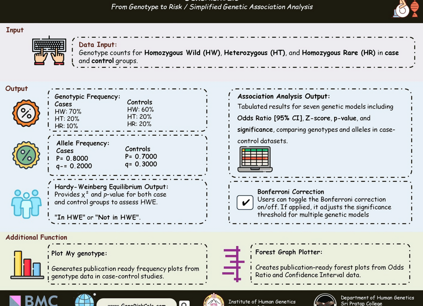
Input/ output specification
GeneRiskCalc requires genotypic counts for Homozygous Dominant (HW), Heterozygous (HT), and Homozygous Recessive (HR) in both case and control groups. These values are used for HWE analysis and OR calculation with a 95% CI and p-value.
Concerning the Output, the results will include genotypic frequency, allele frequency, HWE status based on χ2 value, p-value (assessing genetic equilibrium), and OR/CI with p-value (indicating genetic association strength). For visualization, users can manually input OR and CI values or copy data from Excel into the integrated Forest Plotter to illustrate effect size and direction.
Data visualization
The results are displayed in a structured table, presenting clear and organized information on key statistical measures, including allele and genotype counts, HWE with χ2 and p-values, and OR with 95% CI, and p-values. Additionally, Bonferroni correction is applied for multiple genetic models to ensure accuracy.
Validation of GeneRiskCalc
The accuracy and reliability of GeneRiskCalc were rigorously validated through multiple approaches. Benchmark testing compared results with established tools to ensure precision. For HWE analysis, various online software were used such as bio. blog.labs (Seb Carvello—Hardy–Weinberg Equilibrium Calculator), Wpcalc (Online Calculator of Hardy–Weinberg equilibrium), San Mateo (Excel file: Supplementary file-1).
Furthermore, to validate and compare the calculated ORs, several freely available online tools were utilized. These included MedCalc’s Odds Ratio Calculator (https://www.medcalc.org/calc/odds_ratio.php), GIGA Calculator’s Odds Ratio tool (https://www.gigacalculator.com/calculators/odds-ratio-calculator.php), the OpenEpi 2 × 2 Table Statistics tool (OpenEpi–2 × 2 Table Statistics), and the Odds Ratio calculator provided by Epitools (https://epitools.ausvet.com.au/twobytwotable). These platforms facilitated cross-verification of OR values and supported a robust interpretation of the statistical results.
To ensure result consistency, simulated datasets with predefined HWE status (Table 2) and OR values were analyzed (Table 3). Additionally, real-world genetic association datasets were tested to validate performance in practical scenarios (Table 4). The tool’s robustness was further assessed by evaluating edge cases, including scenarios with zero genotype counts and extreme OR values (Table 2). Finally, user interface testing was conducted to ensure seamless data input, intuitive result interpretation, and overall ease of use. Together, these validation steps confirm that GeneRiskCalc delivers accurate, reliable, and robust results for genetic association analysis. The workflow of GeneRiskCalc, from data input to result visualization, is depicted in Fig. 1.
Table 2 Comparison of Hardy–Weinberg equilibrium calculations across different tools using simulated dataTable 3 Validation of GeneRiskCalc against other OR calculation tools using randomly selected simulated dataTable 4 Data validated for odds ratio under different genetic modelsFig. 1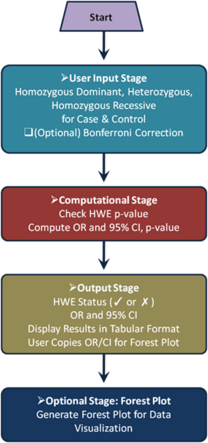
Workflow diagram of GeneRiskCalc from input to visualization: The process includes user data entry, Hardy–Weinberg Equilibrium testing, Odds Ratio calculation, and optional forest plot generation for result visualization