Quantum non-unitary time evolution
QNUTE is a quantum algorithm that simulates the dynamics of the Schrödinger equation with an arbitrary non-Hermitian Hamiltonian \({\hat{H} = \sum _{m=1}^M i\hat{h}_m}\), where each \(\hat{h}_m\) is a local operator which may be non-Hermitian. The non-unitary time evolution operator generated by \(\hat{H}\) is approximated by its first order Trotter product, and takes the form
$$\begin{aligned} e^{-i\hat{H}T} \approx \left( \prod _{m=1}^M e^{\hat{h}_m \Delta t}\right) ^{N_T}, \end{aligned}$$
(6)
where \(N_T = T/\Delta t\)19,20. The normalised actions of each Trotter step \(e^{\hat{h}_m\Delta t}\) acting on a state \(\vert \psi \rangle\) are approximated with unitaries of the form \(e^{-i\hat{A}\Delta t}\), and implemented with Trotter products of the form
$$\begin{aligned} e^{-i\hat{A}\Delta t} \approx \prod _{I=1}^{\mathcal {I}} e^{-i a_I \hat{\sigma }_I \Delta t}. \end{aligned}$$
(7)
In Eq. (7), \({\hat{A}=\sum _{I=1}^{\mathcal {I}} a_I \hat{\sigma }_I}\) is a Hermitian operator with \(\hat{\sigma }_I\) denoting Hermitian operators chosen such that each unitary \(e^{-i \theta \hat{\sigma }_I }\) is efficiently implemented with a quantum circuit parameterised by \(\theta\). The real-valued coefficients \(a_I\) are determined by minimising the expression
$$\begin{aligned} \left\| \frac{e^{\hat{h}_m \Delta t}\vert \psi \rangle }{\sqrt{ \langle {\psi }\vert {e^{\hat{h}_m^\dagger \Delta t} e^{\hat{h}_m \Delta t}}\vert {\psi }\rangle }} – e^{-i\hat{A}\Delta t}\vert \psi \rangle \right\| , \end{aligned}$$
(8)
up to \(O(\Delta t)\), which involves solving a system of linear equations, \({(S+S^\top )\, \vec {a}=\vec {b}}\), constructed using various measurements on \(\vert \psi \rangle\). In particular, we have
$$\begin{aligned} S_{I,J} = \langle {\psi }\vert {\hat{\sigma }_I^\dagger \hat{\sigma }_J}\vert {\psi }\rangle , \quad c = \sqrt{1 + 2\Delta t\, \text {Re} \langle {\psi }\vert {\hat{h}_m}\vert {\psi }\rangle }, \quad b_I = \frac{-2}{c}\, \text {Im} \langle {\psi }\vert {\hat{\sigma }_I^\dagger \, \hat{h}_m}\vert {\psi }\rangle , \end{aligned}$$
(9)
see Supplementary Information for further details on the construction. Simulating each Trotter step involves taking \(O(\mathcal {I}^2)\) measurements to construct the \(\mathcal {I}\times \mathcal {I}\) matrix equation and generates a quantum circuit of depth \(O(\mathcal {I})\). The full simulation therefore requires \(O(N_T M \mathcal {I}^2)\) measurements.
The states generated by QNUTE are determined by the choice of \(\hat{\sigma }_I\). For example, choosing \(\hat{\sigma }_I\) to encompass all Pauli strings allows us to capture arbitrary state vector rotations in the state space, whereas restricting \(\hat{\sigma }_I\) to Pauli strings involving an odd number of \(\hat{Y}\) gates significantly reduces the operator decomposition count and allows us to capture those rotations that do not introduce complex phases to the quantum state. Given a choice of \(\hat{\sigma }_I\), the accuracy of the QNUTE implementation is dependent on the support of \(\hat{A}\). Ideally, the support of \(\hat{A}\) should cover \({D=O(C)}\) adjacent qubits surrounding the support of \(\hat{h}_m\), where the correlation length C denotes the maximum distance between interacting qubits in the Hamiltonian. However, our choice to express \(\hat{A}\) has been in terms of Pauli strings, which gives rise to an exponential dependence on D, \({\mathcal {I}=O(2^D)}\). For this reason, we have considered an inexact implementation of QNUTE that uses a constant domain size \(D.
We will demonstrate that QNUTE can be used to approximate solutions to arbitrary linear PDEs with solutions stored in the qubit state vector. Information relevant to the solution is extracted by taking measurements on the final quantum state. It is expected that the number of distinct measurements required to extract the relevant information should scale polynomially with the number of qubits. Further, if it is known that the solution to a PDE will be real-valued and non-negative, then the normalised solution calculated by QNUTE can be extracted obtained by taking the square root of the probability distribution of computational basis states. We will use QNUTE to simulate the Black-Scholes equation, as it has a non-Hermitian Hamiltonian and has non-negative real-valued solutions.
Simulating black-scholes with QNUTE
To model the dynamics of the Black-Scholes equation, we discretise the domain \([x_0,x_N]\) into \(2^n\) points equally spaced by a distance of \(h = \frac{x_N – x_0}{2^n – 1}\). The normalised samples of the option price are stored in an n-qubit quantum state given by
$$\begin{aligned} \vert \bar{u}(\tau )\rangle = \frac{\sum _{k=0}^{2^n-1} u(x_k, \tau ) \vert k\rangle }{\sqrt{\sum _{k=0}^{2^n-1} u^2(x_k, \tau ) }}, \end{aligned}$$
(10)
where \(x_k = x_0 + kh\). Following Eq. (5), the discretised Black-Scholes Hamiltonian can be represented in terms of a central finite difference matrix of the form
$$\begin{aligned} -i\hat{H}_{BS} = \begin{bmatrix} \gamma _0 & \beta _0 & & \\ \alpha _1 & \gamma _1 & \beta _1 & \\ & \ddots & \ddots & \ddots & & \\ & & \alpha _{2^n-2} & \gamma _{2^n-2} & \beta _{2^n-2} \\ & & & \alpha _{2^n-1} & \gamma _{2^n-1} \end{bmatrix}, \end{aligned}$$
(11)
where
$$\begin{aligned} \alpha _k = \frac{\sigma ^2 x_k^2}{2h^2} – \frac{r x_k}{2h}, \quad \beta _k = \frac{\sigma ^2 x_k^2}{2h^2} + \frac{r x_k}{2h} \quad \text {and} \quad \gamma _k = -r – \alpha _k – \beta _k. \end{aligned}$$
(12)
Refer to Supplementary Information for the representation of the discretised Hamiltonian of Eq. (11) in the Pauli operator basis.
Norm correction
The scale factor c given in Eq. (9) approximates how the Trotter step scales \(\vert \psi \rangle\) up to \(O(\Delta t)\). These approximations can be stored and multiplied to provide an approximation of how the state vector scales over the course of the evolution. Excluding the scenario of the ideal implementation of QNUTE that records a perfect fidelity, errors associated to each scale factor will compound over multiple Trotter steps, which must be corrected periodically. For an anti-Hermitian Hamiltonian \(\hat{H}=i\hat{L}\), it was shown that the correction factor can be calculated using knowledge of the non-degenerate ground state \(\vert \psi _0\rangle\) of \(\hat{L}\) and its corresponding eigenvalue \(\lambda _0\)18. This correction strategy necessarily exploits the mutual orthogonality of the eigenstates of the associated Hamiltonian.
However, since the discretised Black-Scholes Hamiltonian as given in Eq. (11) is not a normal operator, its eigenvectors are not guaranteed to be mutually orthogonal. This, therefore, rules out the norm correction strategy pursued in Ref.18. Interestingly, variational QITE has been employed as a technique for solving the Black-Scholes equation. Under this setting, the normalisation factor was considered either as a variational parameter5 or was determined with prior knowledge of how, specifically, call option prices evolve at the boundary \(x_N\)3. Since the former is not compatible with QNUTE, we generalise the latter approach to cater to various European option types.
Consider the Black-Scholes equation, as given in Eq. (5), with option price \(u(x,\tau )\) assumed to be linear in x in the neighbourhood of the boundaries \(x_0\) and \(x_N\). We will consider linear boundary conditions, since they are widely used in classical option pricing simulations and are known to be numerically stable21. Thus, under linear boundary conditions, the option price takes the form \({u(x,\tau ) = a(\tau )x + b(\tau )}\) near the boundaries. Substituting this form into Eq. (5) reduces the Black-Scholes equation to an ordinary differential equation (ODE) at the boundaries
$$\begin{aligned} x\frac{{\textrm{d}}a}{{\textrm{d}}\tau } + \frac{{\textrm{d}}b}{{\textrm{d}}\tau } = -rb(\tau ). \end{aligned}$$
(13)
Solving Eq. (13) yields \(a(\tau ) = a(0)\) and \(b(\tau ) = b(0)e^{-r\tau }\), where a(0), and b(0) can be derived from the initial conditions p(x) at each boundary. If a(0) or b(0) are non-zero on at least one of the boundaries, we can rescale a normalised solution to ensure that the value at that boundary is equal to \(a(\tau )x+b(\tau )\).
To guarantee that the linear boundary conditions apply during the QNUTE simulation, they must be encoded into the Black-Scholes Hamiltonian. The first and last rows of the matrix in Eq. (11) are updated with the corresponding forward and backward first-order finite difference coefficients, respectively, with the second-derivative terms vanishing as the function is linear. The Black-Scholes Hamiltonian inclusive of linear boundary conditions takes the form
$$\begin{aligned} -i\hat{H}_{LBS} = \begin{bmatrix} \gamma _0^\prime & \beta _0^\prime & & \\ \alpha _1 & \gamma _1 & \beta _1 & \\ & \ddots & \ddots & \ddots & & \\ & & \alpha _{2^n-2} & \gamma _{2^n-2} & \beta _{2^n-2} \\ & & & \alpha _{2^n-1}^\prime & \gamma _{2^n-1}^\prime \end{bmatrix}, \end{aligned}$$
(14)
where
$$\begin{aligned} \gamma _0^\prime =\ -r – \frac{r x_0}{h}, \quad \beta _0^\prime =\ \frac{r x_0}{h}, \quad \alpha _{2^n-1}^\prime =\ -\frac{r x_N}{h}, \quad \text {and} \quad \gamma _{2^n-1}^\prime =\ -r + \frac{r x_N}{h}. \end{aligned}$$
(15)
See Supplementary Information for the Pauli decomposition of this Hamiltonian.
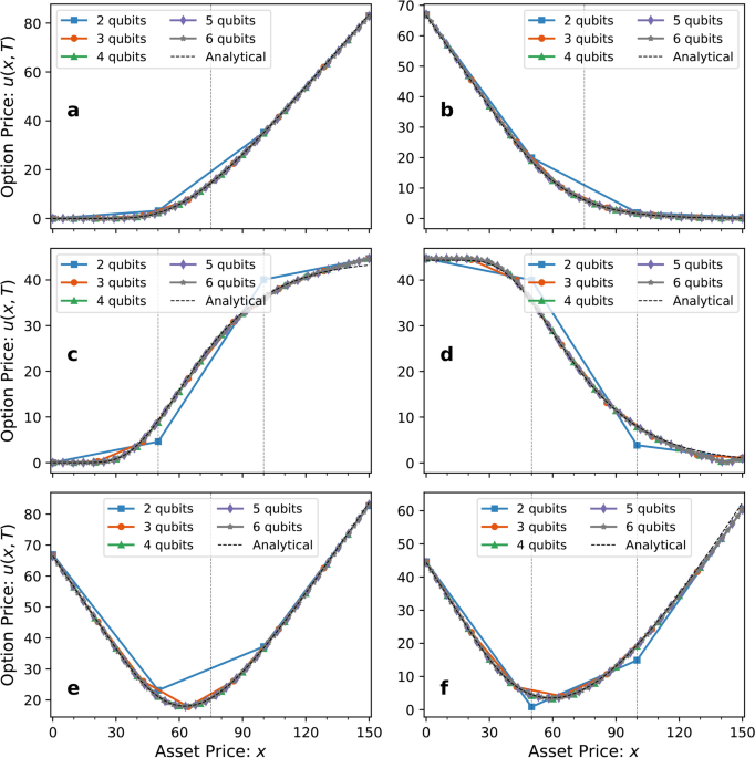
Fig. 1
Black-Scholes option pricing simulations using QNUTE. The figure compares the Black-Scholes option prices calculated using QNUTE with varying number of qubits to the corresponding analytical solutions for the following European option types: (a) Call (b) Put (c) Bull Spread (d) Bear Spread (e) Straddle (f) Strangle. The vertical dashed lines at \(x=50,75,\) and 100 correspond to the strike prices of the option contracts. We simulated the solutions for the asset prices \(x\in [0,150]\), with the maturity time \(T=3\) years, simulated over \(N_T=500\) time steps. Our simulations used a risk-free interest rate of \(r=0.04\), and the volatility \(\sigma =0.2\). The unitaries used to approximate the evolution act on all of the qubits used in the simulation.
Fig. 2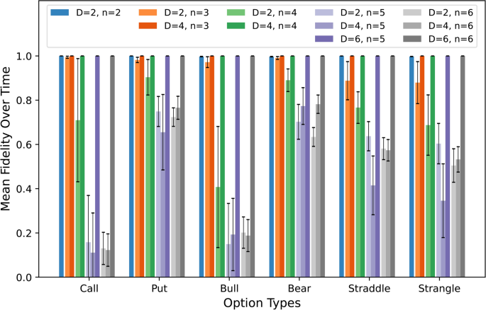
Average fidelities of inexact QNUTE implementations. The figure shows the fidelities of different implementations of inexact QNUTE used to simulate Black-Scholes dynamics averaged over each time step, with the error bars depicting the standard deviation. These simulations share the same parameters values for \(r,\sigma ,T\) and \(N_T\) as with the simulations shown in Fig. 1. n denotes the number of qubits used to store the function samples, and D denotes the maximum number of adjacent qubits targeted by the unitaries. The overall low fidelities shown the by inexact QNUTE, where \(D, indicate that the Black-Scholes Hamiltonian with linear boundary conditions has a high correlation length, making it difficult to accurately reproduce its evolution with small unitaries.