Formalism
We extend the Kane-Mele model by including a collinear AFM order which is exchange coupled to the electrons on a 2D honeycomb lattice. As illustrated in Fig. 1, the magnetic moments on the A and B sublattices are oppositely aligned and pointing perpendicular to the plane. The conceived system is characterized by an effective tight-binding Hamiltonian
$$H=\, t \sum_{\langle i,j\rangle }{c}_{i}^{{\dagger} }{c}_{j}+i{\lambda }_{soc} \sum_{\langle \langle i,j\rangle \rangle }{\nu }_{ij}{c}_{i}^{{\dagger} }{s}_{z}{c}_{j}+i{\lambda }_{R} \sum_{\langle i,j\rangle }{c}_{i}^{{\dagger} }{({{\bf{s}}}\times {\hat{{{\bf{d}}}}}_{ij})}_{z}{c}_{j}\\ +{\lambda }_{v} \sum_{i}{c}_{i}^{{\dagger} }{\xi }_{i}{c}_{i}+{\lambda }_{ex} \sum _{i}{c}_{i}^{{\dagger} }({{{\bf{m}}}}_{i}\cdot {{\bf{s}}}){c}_{i},$$
(1)
where \({c}_{i}^{{\dagger} }({c}_{i})\) is the electron creation (annihilation) operator on site i, with the spin index omitted for succinctness. In Eq. (1), the first term represents the nearest neighbor hopping. The second term is the intrinsic SOC which affects the next-nearest neighbor hopping, where \({\nu }_{ij}=2/\sqrt{3}{({\hat{{{\bf{d}}}}}_{1}\times {\hat{{{\bf{d}}}}}_{2})}_{z}=\pm 1\) with \({\hat{{{\bf{d}}}}}_{1}\) and \({\hat{{{\bf{d}}}}}_{2}\) being the two unit vectors along the 120∘ bonds connecting i and j. The third term is the Rashba SOC arising from the broken mirror symmetry (with z normal), where \({\hat{{{\bf{d}}}}}_{ij}\) is the unit vector connecting the nearest-neighboring sites i and j, and s is the vector of Pauli matrices for the spin degree of freedom. The fourth term is the staggered potential where ξi = ±1 flips sign on the A and B sublattices as shown in the Fig. 1, breaking the C2 symmetry about the x axis. The last term represents the exchange coupling between the electrons and the local magnetic moments, where \({{{\bf{m}}}}_{i}=\pm \hat{{{\bf{z}}}}\) is the unit magnetic vector on site i.
Fig. 1: Schematic of a honeycomb lattice with G-type AFM order.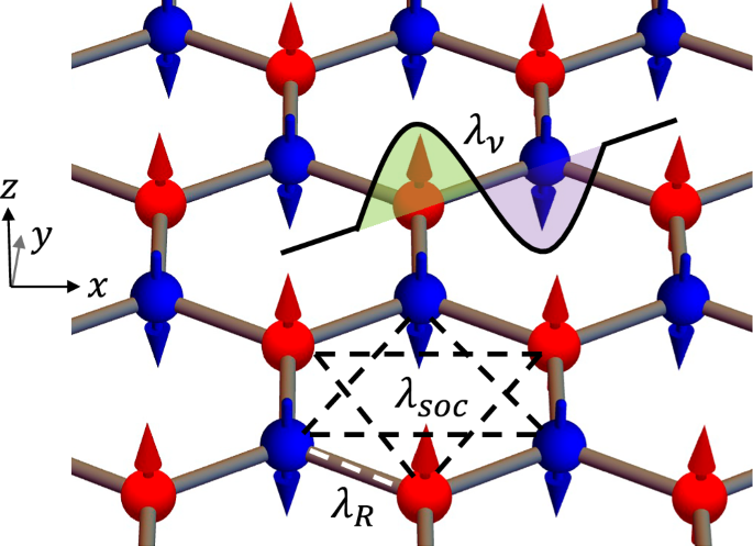
The wavy potential well represents the staggered potential on A and B sublattices. The intrinsic SOC and Rashba SOC introduce extra phases in the nearest neighbor (white dashed line) and next nearest neighbor hopping (black dashed line), respectively. The coordinates axis are shown on the left.
Topological phases
If the exchange coupling λex vanishes, the Hamiltonian preserves the time-reversal symmetry. Then for a sufficiently large λsoc, the system can exhibit the QSH phase characterized by the Z2 number19. Now, with a finite λex, the time-reversal symmetry is broken so the Z2 number becomes ill-defined. Moreover, the QSH phase has a vanishing Chern number (C = 0), so it could only be distinguished from the normal insulator (NI) phase by the spin Chern number Cs = (C↑ − C↓)/231,32.
We first draw the phase diagrams of the Chern number C in Fig. 2a, b by navigating λsoc, λv and λR. To ensure a proper quantization of the topological invariant, we impose an upper limit of 0.1t for the values of λsoc, λR, λex and λv so as to maintain a global band gap. We find three distinct phases on these two diagrams. The QSH state only appears at large λsoc. At λv = 0, the threshold of QSH is about λsoc = ±0.03t. Two observations are in order. First, different from the QSH state, the QAH state requires a nonzero staggered potential λv. This is because the staggered potential breaks the \({{\mathcal{PT}}}\) symmetry (combined inversion and time reversal), enabling a non-zero Berry curvature33,34,35. Second, while the Chern number flips sign when either λv or λsoc flips sign, it remains the same regardless of λR, because +λR and −λR are related by a mirror reflection z → −z, which does not change the sign of C. In Fig. S1, we also provide the phase diagrams for other combinations of parameters (e.g., λsoc and λex). We conclude that the sign of the total Chern number is determined by sign[C] = sign[λsoc]sign[λv]sign[λex].
Fig. 2: Electronic phase diagrams and edge states.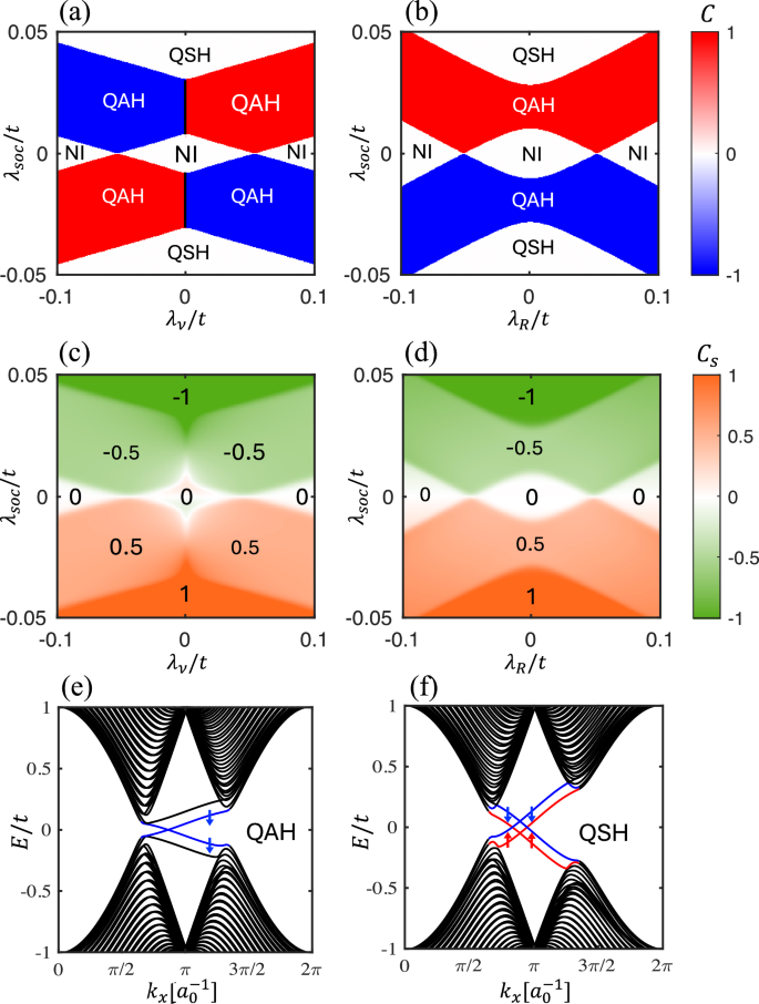
Chern number (a, b) and spin Chern number (c, d) with respect to intrinsic SOC strength λsoc for different staggered potential and Rashba SOC strength λR. In a, c, λR is fixed to be 0.05t. In b, d, λv is fixed to be 0.05t. Band structure of a finite system, with 40 unit cells in the y direction, for e λsoc = 0.02t and f λsoc = 0.05t. In both e, f, λR = 0.025t and λv = 0.05t. The edge states in the bulk band gap are colored blue or red depending on the spin polarization. a0 is the lattice constant. In all cases, λex = 0.1t.
We next plot the phase diagrams of the spin Chern number Cs in Fig. 2c, d, corresponding to the results in Fig. 2a, b, respectively. As expected, Cs in the QSH state is quantized to be ±1. In the QAH state, however, Cs is quantized to be ±0.5, which indicates that the chiral edge electrons only carry one spin species (see Fig. S2 for further details). It is important to note that the spin Chern number near the phase boundaries is not exactly quantized or half quantized, because the spin is not a strictly conserved quantity in the presence of a finite Rashba SOC. Concerning the sign flip of Cs, we observe a quite different pattern as compared to C. For example, Cs is even in λv while being odd in λsoc. This can be understood from definition of spin currents: if the spin polarization and the flowing direction both flip sign, a spin current will remain unchanged.
To further confirm the system topology revealed by the phase diagrams, we plot in Fig. 2e, f the band structures of our Hamiltonian truncated in the y direction with N = 40 unit cells (i.e., a nanoribbon periodic only in the x direction). For λsoc = 0.02t, the system is in the QAH state, where only one pair of chiral edge states with the same spin polarization but opposite group velocities emerges in the band gap. For λsoc = 0.05t, the system transitions into the QSH phase, where two pairs of chiral edge states appear in the bulk gap with opposite spin polarizations.
Néel-type spin-orbit torque
Having obtained the band topology with broken time-reversal symmetry introduced by the AFM order, we are in a good position to explore the interplay between electron transport and magnetic dynamics. For insulating systems where the ordinary spin Hall effect is suppressed, applying an (in-plane) electric field E can directly generate non-equilibrium spin accumulation through the Edelstein effect36. The induced spin accumulation can in turn excite magnetic dynamics through the SOT37,38,39,40. In our context, it is important to discern different AFM sublattices in the non-equilibrium spin generation. While the average component δS = (δSA + δSB)/2 (due to the Edelstein effect) leads to the ordinary SOT, the contrasting component δN = (δSA − δSB)/2 (due to the staggered Edelstein effect) leads to the NSOT25. As we consider insulating magnets where the Fermi energy εF lies in the bulk gap, δS and δN only involve the Fermi-sea contribution. Within the linear response regime, we can express the contrasting spin accumulation as25,39,41
$$\delta {{\bf{N}}}=\frac{e{\hslash }^{2}}{2} \sum_{{\epsilon }_{n}
(2)
where v is the velocity operator and Γ is the energy broadening due to disorder. The average spin accumulation δS follows a similar formula with the pseudo-spin Pauli matrix (acting on the sublattices) τ3 replaced by the identity matrix. Unlike the Fermi-level contribution, here δN does not diverge even in the clean limit Γ → 0 where Eq. (2) reduces to a formula similar to the spin Chern number [see Eq. (8)]. In the following, we will take representative values for the exchange interaction λex = 0.1t = 100 meV and for the band broadening Γ = 20 meV.
Without sacrificing generality, we set the E field in the x direction and calculate the non-equilibrium spin accumulation on each sublattice: δSA = (δS + δN)/2 and δSB = (δS − δN)/2. Figure 3a, b plot \(\delta {S}_{x}^{A}\) and \(\delta {S}_{x}^{B}\) as functions of λsoc and λR, while the y and z components are found to be zero. Remarkably, we find that \(\delta {S}_{x}^{A}\) and \(\delta {S}_{x}^{B}\) are exactly opposite to each other so long as λv = 0, meaning that only the NSOT exists whereas the SOT vanishes (i.e., δS = 0). As a consistency check, the way δSA(B) varies over the direction of E is shown in Fig. S4, where the contrasting feature \(\delta {S}_{x(y)}^{A}=-\delta {S}_{x(y)}^{B}\) persists. Figure 3c, d schematically show the difference between the SOT and NSOT, driven by δSA = δSB and δSA = −δSB, respectively. In the clean limit Γ → 0, the spin accumulation on each sublattice is directly related to the Berry curvature residing in the mixed space of crystal momentum and magnetization13,17:
$$\delta {S}_{\nu }^{A(B)}=\frac{e\hslash }{2{\lambda }_{ex}}{E}_{\mu }\left\langle {\Omega }_{\mu \nu }^{k{m}^{A(B)}}\right\rangle,$$
(3)
where 〈 ⋯ 〉 = Vuc/(2π)2∑n∫d2kf[εn(k)]( ⋯ ) denotes the average over the first Brillouin zone with Vuc the unit cell volume (area) and the f the Fermi distribution. For Γ ≠ 0, the Berry curvature is dressed by the broadening Γ, becoming the integrand of Eq. (2). For λv = 0, the Berry curvature assumes a staggered pattern \({\Omega }_{\mu \nu }^{k{m}^{A}}=-{\Omega }_{\mu \nu }^{k{m}^{B}}\), hence δSA = −δSB. A non-zero λv would render \(| \delta {S}_{x}^{A}| \ne | \delta {S}_{x}^{B}|\) owing to the introduction of staggered potentials on the sublattices (see Fig. S3), which leads to a finite δS on top of the δN, hence inducing a nonzero SOT besides the NSOT.
Fig. 3: Non-equilibrium spin accumulations and their ensuing torques.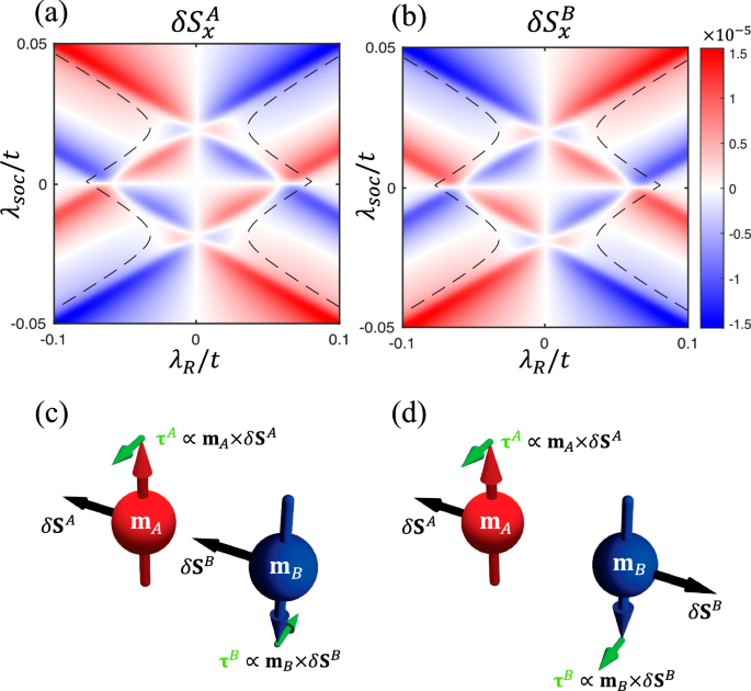
a, b Phase diagrams of δS per unit cell (in units of ℏ/2) for each sublattice induced by Ex = 1V/μm for λv = 0. The dashed lines mark where the global band gap is reduced to 1 meV with an increasing ∣λR∣. Illustrative comparison between: c ordinary SOT induced by a uniform spin accumulation δSA = δSB, and d NSOT induced by a contrasting spin accumulation δSA = −δSB.
In the phase diagram, the dashed lines mark where the global gap reduces to 1 meV. For a large ∣λR∣ beyond these boundaries, the global gap will be smaller than 1 meV, making it difficult to restrict εF in the gap and, more seriously, less practical to guarantee the adiabatic condition (to be clear in the next section). Therefore, we should focus on the central region of Fig. 3a, b enclosed by the dashed lines to safely ignore the Fermi-surface contribution to δSA(B).
The NSOT is known for being able to switch the Néel order n = (mA − mB)/2 in non-centrosymmetric AFM metals25,26,27,28,29,30. But previous experimental studies are limited to current-induced NSOT. By contrast, our predicted NSOT is in principle free of dissipation because it is mediated by the adiabatic motions of valence electrons, incurring no Ohm’s current as no conduction electrons are involved in the generation of spin torques. The adiabatic origin of the NSOT, similar to the SOT previously claimed in iMTIs, is also reflected by its Berry-curvature origin discussed above. We emphasize that the Berry curvature Ωkm relevant to the NSOT is physically distinct from the momentum-space Berry curvature Ωkk that determines the band topology12,16.
To better clarify this subtle point, we plot in Fig. 4a the sublattice spin accumulations δSA and δSB as functions of λsoc with vanishing λv = 0, i.e., a vertical cut at λR = 0.02t in Fig. 3. As a comparison, we also plot the results with a non-vanishing staggered potential λv = 0.04t in Fig. 4b. The NI, QAH and QSH regions are shaded in light green, purple and orange, respectively. Three key observations are in order. First, although δSA,B turn out to be slightly larger in the QAH and QSH states, they remain finite even in the topologically trivial phase, suggesting that the NSOT cannot be fully characterized by the band topology. Second, δSA,B exhibit sudden jumps at the QAH-NI and QSH-NI transitions. These jumps would formally diverge in the clean limit Γ → 0 due to gap closing; but in our plots, a finite Γ = 20 meV is added to suppress the divergence. Third, the hallmark NSOT signature, \({{\rm{sgn}}}(\delta {{{\bf{S}}}}^{A})=-{{\rm{sgn}}}(\delta {{{\bf{S}}}}^{B})\), is most robust in the QSH phase. While a finite λv enables a QAH phase interpolating the QSH and NI phases in Fig. 4b, it also imbalances the potentials on the two sublattices, rendering δSA and δSB different in magnitude. Specifically, we have \(\delta {S}_{x}^{A}/\delta {S}_{x}^{B}\approx -1.28\) at λsoc = 0.05t, whereas in Fig. 4a with λv = 0 we have exactly \(\delta {S}_{x}^{A}/\delta {S}_{x}^{B}=-1\) for all λsoc. The dependencies of δSA,B on λR and λex are shown in Fig. S3.
Fig. 4: Non-equilibrium spin accumulations across different phases.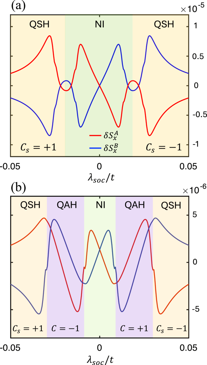
δS per unit cell (in units of ℏ/2) for each sublattice as a function of λsoc with a λv = 0 and b λv = 0.04t. For each topological nontrivial regions, the corresponding Chern number or spin Chern number are labeled in the bottom. In both figures, we adopt λR = 0.02t, λex = 0.1t = 100 meV, Ex = 1V/μm.
Electric field-driven antiferromagnetic resonance
To demonstrate the dynamical consequences of the predicted NSOT, we now study the AFM resonance driven by an AC electric field. In terms of the unit vectors of the sublattice magnetic moments, the governing Landau-Lifshitz-Gilbert (LLG) equations are:
$${\dot{{{\bf{m}}}}}^{A}=\gamma \left[-{{{\mathcal{H}}}}_{J}{{{\bf{m}}}}^{B}+{{{\mathcal{H}}}}_{\parallel }({{{\bf{e}}}}_{\parallel }\cdot {{{\bf{m}}}}^{A}){{{\bf{e}}}}_{\parallel }+{{{\bf{H}}}}_{0}+{{{\bf{h}}}}_{D}^{A}\right]\times {{{\bf{m}}}}^{A}+{\alpha }_{0}{{{\bf{m}}}}^{A}\times {\dot{{{\bf{m}}}}}^{A}$$
(4a)
$${\dot{{{\bf{m}}}}}^{B}=\gamma \left[-{{{\mathcal{H}}}}_{J}{{{\bf{m}}}}^{A}+{{{\mathcal{H}}}}_{\parallel }({{{\bf{e}}}}_{\parallel }\cdot {{{\bf{m}}}}^{B}){{{\bf{e}}}}_{\parallel }+{{{\bf{H}}}}_{0}+{{{\bf{h}}}}_{D}^{B}\right]\times {{{\bf{m}}}}^{B}+{\alpha }_{0}{{{\bf{m}}}}^{B}\times {\dot{{{\bf{m}}}}}^{B},$$
(4b)
where γ > 0 is the gyromagnetic ratio, \({{{\mathcal{H}}}}_{J}\) is the AFM exchange field (summed over all nearest neighbors), \({{{\mathcal{H}}}}_{\parallel }\) is the anisotropy field for the easy axis e∥, H0 is the external static field, and α0 is the Gilbert damping constant. For simplicity, let e∥ be the z axis and H0 be applied along e∥, lifting the degeneracy of the AFM resonance modes.
Under a microwave irradiation, the oscillating driving field \({{{\bf{h}}}}_{D}^{A(B)}\) can arise either directly from the magnetic field hrf or indirectly from the NSOT field
$${{{\bf{h}}}}_{{{\rm{NS}}}}^{A(B)}=-\frac{2{\lambda }_{ex}}{\hslash {m}_{s}}\delta {{{\bf{S}}}}^{A(B)}$$
(5)
produced by the electric field Erf, where ms is the sublattice magnetic moment. According to Eq. (2), δSA/B = (δS ± δN)/2 decreases monotonically with an increasing λex because the topological band gap in our model is primarily determined by λex. Consequently, the NSOT field determined by Eq. (5), with a linear dependence on λex in its front factor, remains insensitive to the change of λex. Of the two mechanisms, hrf (hNS) is perpendicular (parallel) to Erf and is the same (opposite) on each sublattice. Based on Maxwell’s equations, a microwave with ∣Erf∣ = 1V/μm has a magnetic field ∣hrf∣ = 33 Gauss. The same electric field can generate a maximum non-equilibrium spin of 0.85 × 10⁻⁵ ℏ per sublattice according to Fig. 3, which converts to an effective NSOT field ∣hNS∣ = 59 Gauss for ms = 5μB. While we are not able to locate a specific material on the phase diagram Fig. 3, it is instructive to chose a point where ∣hrf∣ = ∣hNS∣, so we can determine how their distinct symmetry (uniform hrf versus opposite hNS on the two sublattices) could lead to dramatically different microwave absorptions with the onset of AFM resonance.
To this end, we focus on the point at λsoc = 0.05t, λR = 0.072t, and λv = 0, which lies in the QSH phase. Here, an electric field of 0.5V/μm will produce a staggered spin accumulation \(\delta {S}_{x}^{A}=-\delta {S}_{x}^{B}=-2.4\times 1{0}^{-6}\hslash\) per unit cell (about 64% of the maximum capacity on the phase diagram), which corresponds to hNS = 16.5 G, matching the real magnetic field hrf of the same electromagnetic wave. We then consider a linearly polarized microwave incident from the y direction with either hrf or Erf (hence the hNS), but not both, parallel to the x axis, as illustrated in Fig. 5a, b, respectively. Such experimental conditions can be typically realized with the Voigt geometry rather than the Faraday geometry42. Under the device geometry in Fig. 5a [Fig. 5b], the electric field Erf (magnetic field hrf) is collinear with the magnetic moments so that only hrf (Erf) drives the AFM dynamics, separating the NSOT-induced resonance from the ordinary AFM resonance.
Fig. 5: Antiferromagnetic resonances.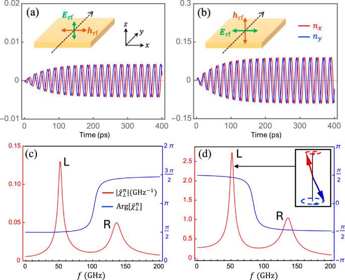
Time evolution of the Néel order n(t) at the resonance of the left-handed mode (with f = 51.9 GHz set by a bias field H0 = 1.5 T) for a hrf-driven configuration, and b Erf-driven configuration. c, d are the corresponding amplitude (red, left axis) and phase (blue, right axis) of the dynamical susceptibility \({\tilde{\chi }}_{\perp }^{n}\) as a function of driving frequency f, where the low-frequency mode is left-handed (inset). Parameters: HJ = 35 T, H∥ = 0.16 T, α0 = 0.005, and Erf = 0.5V/μm (corresponding to hrf = 16.5 Gs).
Next, we study the time evolution of the Néel vector n(t) by numerically solving the LLG equations (4), where parameters are given typical values in 2D honeycomb TMTs (such as MnPS3 and its variances43,44): ms = 5μB, \({{{\mathcal{H}}}}_{J}=35\) T and \({{{\mathcal{H}}}}_{\parallel }=0.16\) T. Figure 5a, b plot the transverse components nx(t) and ny(t) for the two distinct cases under the resonance condition of the low-frequency mode: \(f=\gamma \sqrt{{{{\mathcal{H}}}}_{\parallel }({{{\mathcal{H}}}}_{\parallel }+2{{{\mathcal{H}}}}_{J})}-\gamma {H}_{0}\)45, where H0 = 1.5 T is applied along the +z direction, yielding the low-frequency mode left-handed as illustrated by the inset of Fig. 5d. With our chosen parameters, this H0 field is well below the spin-flop threshold while separating the left-handed and right-handed modes by 84 GHz. We emphasize that the vertical axis in Fig. 5b has a scale 15 times larger than that in Fig. 5a, and the amplitude of AFM resonance is about 20 times larger in Fig. 5b where the magnetic dynamics is activated by the Erf field (through the NSOT). To further confirm this point, we plot in Fig. S5 the case of a vertically incident microwave (i.e., the Faraday geometry) where both hrf and Erf can drive the magnetic dynamics. The result is hardly distinguishable from Fig. 5b, indicating that the NSOT overwhelms the Zeeman coupling in driving the AFM resonance.
If the driving frequency f (in energy scale 2πℏf) is comparable with the band gap18,46, Eq. (2) as a Berry phase result will become invalid because the adiabatic condition is broken and the transitions from the valence band to the conduction band become substantial. But the typical AFM resonance frequency we are considering is at most in the sub-terahertz range, where 2πℏf~0.2 meV is much smaller than the band gap so long as we stay fairly far away from the phase transition point.
Were not the NSOT generation, the electric field Erf is not even able to drive the spin dynamics, let alone entailing an enhanced resonance amplitude. To quantify the resonance absorption of the microwave, we linearlize the LLG equations (4) using the vectorial phasor representation: \({{{\bf{m}}}}^{A(B)}={{\rm{Re}}}[{\tilde{{{\bf{m}}}}}^{A(B)}{e}^{{{\rm{i}}}\omega t}]\) and \({{{\bf{h}}}}_{D}^{A(B)}={{\rm{Re}}}[{\tilde{{{\bf{h}}}}}_{D}^{A(B)}{e}^{{{\rm{i}}}\omega t}]\), with either \({\tilde{{{\bf{h}}}}}_{D}^{A}={\tilde{{{\bf{h}}}}}_{D}^{B}={\tilde{h}}_{{{\rm{rf}}}}\hat{{{\bf{x}}}}\) or \({\tilde{{{\bf{h}}}}}_{D}^{A}=-{\tilde{{{\bf{h}}}}}_{D}^{B}={\tilde{h}}_{{{\rm{NS}}}}\hat{{{\bf{x}}}}\) depending on which component acts as the driving field. Since we have fixed the driving field to be polarized along x, the dynamical susceptibility tensor of the Néel vector reduces to a vector \({\tilde{{{\mathbf{\chi }}}}}_{\perp }^{n}(\omega )=\{{\tilde{\chi }}_{x}^{n}(\omega ),\,{\tilde{\chi }}_{y}^{n}(\omega )\}\) defined by
$${\tilde{n}}_{x(y)}={\tilde{\chi }}_{x(y)}^{n}(\omega )\gamma {\tilde{h}}_{D},$$
(6)
where \({\tilde{h}}_{D}={\tilde{h}}_{{{\rm{rf}}}}\) for the geometry in Fig. 5a, whereas \({\tilde{h}}_{D}={\tilde{h}}_{{{\rm{NS}}}}\) for the geometry in Fig. 5b. For simplicity, we set the initial phase of \({\tilde{h}}_{D}\) zero, so the phase difference between \(\tilde{{{\bf{n}}}}\) and \({\tilde{{{\bf{h}}}}}_{D}\) is embedded in the phase of \({\tilde{{{\mathbf{\chi }}}}}_{\perp }^{n}(\omega )\). We numerically plot the amplitude \(| {\tilde{{{\mathbf{\chi }}}}}_{\perp }^{n}| \equiv \sqrt{| {\tilde{\chi }}_{x}^{n}{| }^{2}+| {\tilde{\chi }}_{y}^{n}{| }^{2}}\) and the phase \({{\rm{Arg}}}[{\tilde{{{\mathbf{\chi }}}}}_{\perp }^{n}]\equiv {{\rm{Arg}}}[{\tilde{\chi }}_{x}^{n}]-{{\rm{Arg}}}[{\tilde{\chi }}_{y}^{n}]\) (in different colors) as a function of the frequency for the hrf-driven resonance and the Erf -driven resonance in Fig. 5c, d, respectively. Similar to the time-domain plots, here we intentionally adopt very different scales for the ordinates in Fig. 5c, d, which clearly shows that \(| {\tilde{{{\mathbf{\chi }}}}}_{\perp }^{n}|\) (hence the microwave absorption) is about 20 times larger when Erf activates the resonance (via the NSOT), as compared with the ordinary hrf-driven mechanism (via direct Zeeman coupling). Basing on \({{\rm{Arg}}}[{\tilde{{{\mathbf{\chi }}}}}_{\perp }^{n}]\), we can further tell that the low-frequency mode indeed exhibits a left-handed precession of the Néel vector while the high-frequency mode is right-handed.
For ferromagnetic resonances47, the power absorption rate at the resonance point is simply proportional to the amplitude of the dynamical susceptibility, given a fixed strength of the driving field. However, the case is subtly different when we turn to AFM resonances and look into the dynamical susceptibility of the Néel vector \({\tilde{{{\mathbf{\chi }}}}}_{\perp }^{n}(\omega )\). Even though we have considered a particular case where hrf = hNS, the actual power absorption rate under the Erf-driven mechanism is not naïvely proportional to \(| {\tilde{{{\mathbf{\chi }}}}}_{\perp }^{n}|\) ascribing to the staggered nature of the NSOT field (\({{{\bf{h}}}}_{{{\rm{NS}}}}^{A}=-{{{\bf{h}}}}_{{{\rm{NS}}}}^{B}\)). In “Method” (Sec. B), we rigorously derive the time-averaged dissipation power for each mechanism, which allows us to quantify the ratio of the microwave power absorption rate under the two mechanisms as \({\bar{P}}_{E}/{\bar{P}}_{H}\approx 438.5\). The significantly enhanced microwave power absorption rate will greatly facilitate the detection of spin-torque excited AFM resonance.
Final remarks
To intuitively understand the pronounced difference in microwave absorption between the two mechanisms, we resort to the symmetry of NSOT. In contrast to the uniform Zeeman field hrf tending to kick mA and mB towards opposite directions, the NSOT field is itself opposite on the two sublattices, \({{{\bf{h}}}}_{{{\rm{NS}}}}^{A}=-{{{\bf{h}}}}_{{{\rm{NS}}}}^{B}\) [see Fig. 3d], which drives the two magnetic moments towards the same direction, thus amplifying their non-collinearity. Consequently, the strong exchange interaction between mA and mB is leveraged to enhance the efficiency of magnetic dynamics, resulting in a much stronger absorption of the microwave.
In summary, we have studied the exotic topological phases, and the spin-torque generations in these phases, based on a G-type AFM material with a honeycomb lattice in the presence of the intrinsic SOC, the Rashba SOC and a staggered potential. We find that the highly non-trivial Néel-type SOT can not only be induced by an applied electrical field without producing Joule heating but also be utilized to drive the AFM resonance at a remarkably high efficiency, which, even under a conservative estimate, is more than one order of magnitude larger than the traditional AFM resonance relying on the Zeeman coupling. Our significant findings open an exciting way for exploiting the unique spintronic properties of AFM topological phases to achieve sub-terahertz AFM magnetic dynamics.