The results of this study are structured to systematically explore the interplay between population mobility and the spread of infectious diseases, using Transfer Entropy (see Fig. 2). The first section analyses the relationship between mobility patterns and COVID19 case data across Spanish provinces, identifying regions that significantly influenced the epidemic’s progression. The second section focuses on the dynamic nature of these interactions, using local or dynamic TE to reveal temporal changes in information flow. In the subsequent section, the impact of non-pharmaceutical interventions is assessed, with the closure of bars and restaurants in Catalunya serving as a case study to illustrate how mobility reductions significantly correlate with the infection trends. Finally, simulated epidemic scenarios validate the framework, demonstrating the critical role of mobility data in avoiding spurious correlations and accurately capturing the drivers of disease spread.
Fig. 2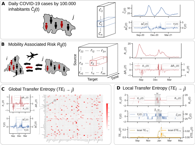
Measuring transfer entropy between time series of phone-based mobility data and incidence to explore patterns of disease spread. Panel A displays the COVID19 incidence \({\hat{C}}_j(t)\) for region j, representing new daily cases per 100,000 inhabitants. This panel also includes the first-order difference \(\Delta {\hat{C}}_j(t)\) and the resulting time series \(Y_j(t)\), derived by discretising \(\Delta {\hat{C}}_j(t)\). Panel B shows the mobility-associated risk between source region i and target region j (\(R_{ij}(t)\)), together with the first-order difference \(\Delta R_{ij}(t)\) and the resulting time series \(X_{ij}(t)\), derived by discretizing \(\Delta R_{ij}(t)\). Panel C illustrates the calculation of the global Transfer Entropy \(TE_{i \rightarrow j}\), which quantifies the information flow between the complete time series \(X_{ij}(t)\) and \(Y_j(t)\) to examine the influence of source region i on the case dynamics in target region j. Panel D illustrates the calculation of the local or dynamic Transfer Entropy \(TE_{i \rightarrow j}(t)\) using sliding windows of size \(\omega\) days to account for the local changes in the flow of information, considering the values of \(X_{ij}(t)\) in the time interval \([t, t+\omega ]\) and the values of \(Y_j(t)\) in the time interval \([t+\delta , t+\delta +\omega ]\). The base map was retrieved from CNIG https://centrodedescargas.cnig.es/CentroDescargas/ under CC-BY 4.0 Licence https://www.ign.es/resources/licencia/Condiciones_licenciaUso_IGN.pdf.
Measuring information flow between mobility patterns and epidemic spread
We used the proposed approach to investigate the role of population mobility in the spread of COVID19 in Spain from 1 March 2020 to 1 May 2021. Phone-based anonymised mobility data was used to compute the mobility-associated risk \(R_{ij}(t)\) between regions and the time series of daily reported cases by 100,000 inhabitants \({\hat{C}}_i(t)\) for the different regions i (see Fig. 2A-B and Datasets for more details). We first focus the analysis at the national level, considering as regions the fifty provinces of Spain and excluding the autonomous cities of Ceuta and Melilla (see Supplementary Fig. S5 and Material and Methods Sections). We measured the global \(TE_{i \rightarrow j}\) between each pair of provinces in Spain (see Fig. 2C). To discretise the time series of mobility-associated risk and daily reported COVID19 cases, we set \(q=1\) (see Calculation of Transfer Entropy between mobility-associated risk and incidence time series for further details on the calculation). The results show that Madrid is the province that exhibits the highest \(TE_{i \rightarrow j}\), which is expected due to fact that Madrid’s high population density, its central location and Madrid city is Spain’s Capital (see Fig. 3A and C and Supplementary Table S1).
Fig. 3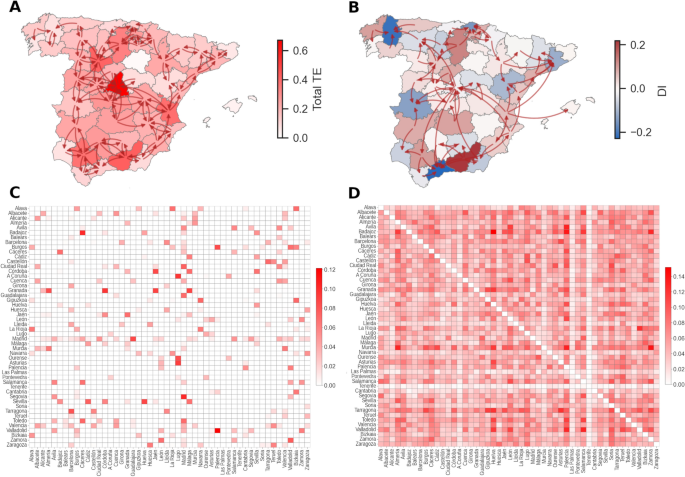
Transfer entropy \(TE_{i \rightarrow j}\) between provinces. Panel A shows the \(TE_{i \rightarrow j}\) between provinces represented by arrows, and the colour of each patch represents the total \(TE_i\) transferred by each province i. Panel B shows the \(DI^{+}_{i \rightarrow j}\) between provinces represented by arrows, and the colour of each patch represents the total \(DI_{i}\) transferred by each province i. In panels A and B, values were filtered using the \(10\%\) percentile from the distribution of the \(\max _j \, TE_{ij}\) and \(\max _j \, DI^{+}_{i \rightarrow j}\), respectively, as explained in the main text. Panels C and D show the Transfer Entropy \(TE_{i \rightarrow j}\) between provinces of Spain, considering and not considering mobility, respectively. TE calculations were performed setting \(\delta =7\) (days) and \(q=1\). The Canary Islands are excluded from Panels A and B due to the absence of measured values for \(TE_{j \rightarrow i}\) and \(DI^{+}_{i \rightarrow j}\). The base map was retrieved from CNIG https://centrodedescargas.cnig.es/CentroDescargas/ under CC-BY 4.0 Licence https://www.ign.es/resources/licencia/Condiciones_licenciaUso_IGN.pdf.
Furthermore, we analysed the directional information difference \(DI^{+}_{i \rightarrow j}\), and total directional information \(DI_{i}\), among provinces (Fig. 3B). The resulting patterns differ markedly from those seen in the analysis of total transfer entropy \(TE_{i \rightarrow j}\) (Fig. 3A). For instance, Madrid, which shows the highest value of total \(TE_{i}\), shows a slightly negative value for the \(DI_{i}\), indicating that the information received by Madrid from other provinces exceeds the amount it transmits to them (Fig. 3B). Comparing province rankings based on \(TE_i\) and \(DI_{i}\) reveals substantial changes, highlighting potential asymmetries in information transfer between neighbouring regions. To further assess this asymmetry, we compared \(TE_{i \rightarrow j}\) and \(TE_{j\rightarrow i}\), finding a significant correlation (\(R=0.62\) and p-value\(=10^{-20}\)) (see Supplementary Fig. S6A), suggesting that information flow between provinces is relatively balanced. However, notable exceptions exist, such as between A Coruña and Lugo, or Asturias and Lugo, where one province exhibits a substantially stronger influence over the other. These cases illustrate instances of pronounced directional influence between regions.
For each source province, we estimate the distribution of the maximum values \(\max _j \, TE_{ij}\) for each province i (see Supplementary Fig. s7). We calculate the \(10\%\) percentile of these maximum values and use it as a threshold to filter out small interactions. After applying this filter, we represent the \(TE_{i \rightarrow j}\) as a directed network on the map, finding that the flow of information primarily occurs between neighbouring provinces (Fig. 3A). Interestingly, the results show almost no Transfer Entropy for certain provinces, including the Canary Islands, the Balearic Islands, and Soria.
To investigate the contribution of mobility in the observed patterns of information flow, we computed the \(TE_{i \rightarrow j}^{cases}\), i.e., the information flow between the time series of cases without considering the mobility (see Calculation of Transfer Entropy between mobility-associated risk and incidence time series). We found significant transfer entropy between almost every pair of provinces (Fig. 3D), suggesting that incorporating mobility helps filter out interactions that may otherwise be confounded or indirect when using case data alone (see Fig. 3C). It is important to note that the presence of significant TE between case time series, even when mobility data is not explicitly considered, does not necessarily indicate misleading or invalid results. Instead, it may reflect dependencies arising from unobserved or indirect mobility pathways, regional synchrony, or shared external influences. Nevertheless, by incorporating direct mobility measurements in the form of the mobility-associated risk, we aim to better resolve the specific pathways through which inter-regional influence occurs, thereby enhancing the interpretability of the observed information flow and grounding it in known mechanisms of disease transmission. We also compared the asymmetry between \(TE_{i \rightarrow j}^{cases}\) and \(TE_{j\rightarrow i}^{cases}\) and observed a remarkable reduction in the correlation coefficient (\(R=0.19\)), emphasizing the critical role of mobility in shaping these dynamics (see Supplementary Fig. S6B). This decrease in symmetry suggests that case-only time series reflect more indirect or confounded dependencies, whereas mobility-informed TE captures more balanced, bidirectional influence patterns, as expected from the generally reciprocal nature of human mobility between regions
We further examined the relationship between inter-provincial distances and \(TE_{i \rightarrow j}\), finding a negative correlation \(R=-0.56\) where \(TE_{i \rightarrow j}\) decays with distance (see Supplementary Fig. S8A). This result is expected since the average number of trips \(M_{ij}\) also shows a negative relation with distance (see Supplementary Fig. S8C). If the analysis is performed between distance and \(TE_{i \rightarrow j}^{cases}\), we found that the correlation coefficient drops to \(R=-0.24\) (see Supplementary Fig. S8B). To address potential biases in Transfer Entropy calculations arising from the potentially limited sample size, we conducted a complementary analysis using Effective Transfer Entropy \(ETE_{i \rightarrow j}\). The results from \(ETE_{i \rightarrow j}\) were consistent with those from \(TE_{i \rightarrow j}\) (see Fig. 3C and Supplementary Fig. S9), as expected given the strong correlation between \(TE_{i \rightarrow j}\) and \(ETE_{i \rightarrow j}\) (see Supplementary Fig. S10). We also computed the \(ETE_{i \rightarrow j}^{cases}\) and found that even with the correction, there is still information flow between almost every pair of provinces (see Supplementary Fig. S11).
Finally, we performed a sensitivity analysis and confirmed that the observed TE and ETE patterns are robust to changes in the delay parameter \(\delta\) days and the discretisation threshold q (see Supplementary Fig. S1, S2, S3 and S4), with optimal and stable results obtained around \(\delta = 7\) days and \(q \approx 1\) (see Supplementary section Sensitivity Analysis of TE and ETE to Parameters \(\delta\)and q). Overall, these results suggest that incorporating mobility data into TE analysis not only improves the interpretability of inter-regional influence but also helps eliminate misleading correlations present in case-only analyses.
Temporal dynamics of mobility-driven information flow
Having established the existence of directional information flow between provinces through global TE measures, we next sought to explore how these relationships evolved by analyzing the dynamic (local) TE. To capture these temporal changes, we measured the dynamic, or local, \(TE_{i \rightarrow j}(t)\) using a day sliding window of length \(\omega\) days with a lag of \(\delta\) days between the time series to account for the virus’s incubation period and symptom onset delay (see Fig. 2D and the subsection Calculation of Transfer Entropy between mobility-associated risk and incidence time series from Material and Methods). We computed both the standard and effective versions of local \(TE_{i \rightarrow j}(t)\), using \(\omega =28\) days, \(\delta =7\) days, and \(q=1\), consistent with the parameters for global \(TE_{i \rightarrow j}\). The resulting TE values are assigned to the end of the window, i.e., time \(t+\omega\), to reflect that the measured TE value is linked to the full time interval rather than a precise time point.
Figure 4 presents the time profiles of local \(TE_{i \rightarrow j}(t)\) calculated between Barcelona and the Balearic Islands as well as in the opposite direction. The results indicate that, for most of the study period, no significant information flow exists between the two provinces. However, in late October, there is a notable peak in information flow from Barcelona to the Balearic Islands, and another peak occurs in February in the reverse direction. Interestingly, both peaks correspond to an increase in \(R_{ij}(t)\), followed by a rise in new cases in the receiving region. Additionally, the timing of these peaks is consistent between both TE and ETE measurements.
Fig. 4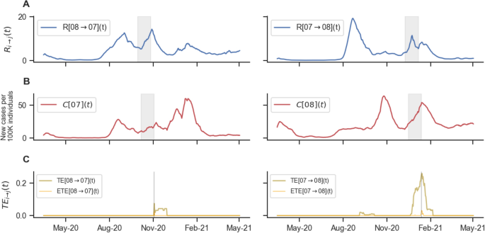
Dynamics \(TE_{i \rightarrow j}\) profiles. Panel A shows \(R_{ij}(t)\) between Barcelona and Baleares on the left and in the opposite direction on the right. Panel B shows the normalized new cases for Barcelona (left) and Baleares (right). Panel C shows the \(TE_{i \rightarrow j}\) and \(ETE_{i \rightarrow j}\) from Barcelona to Baleares (left) and from Baleares to Barcelona. The shaded areas in panels A and B represent the sliding windows for which the TE reaches its maximum value. Transfer Entropy was computed setting \(\delta =7\) days and \(q=1\); for the dynamic TE, we set the length of the sliding window \(\omega\) to 28 days. \(ETE_{i \rightarrow j}\) was computed used \(n=500\) shuffles on \(X_{ij}(t)\).
To assess consistency, we compared global and dynamic \(TE_{i \rightarrow j}\) by taking the time average of dynamic \(TE_{i \rightarrow j}(t)\). The results show a high correlation between global and dynamic TE measurements, with correlation coefficients of 0.86 for standard TE and 0.76 for effective ETE (see Supplementary Fig. S12). This strong correlation indicates that while the global TE still captures the total information flow, the dynamic TE provides insight on the temporal profile for the information flow. This also indicates that the size of the sliding windows, i.e. \(\omega =28\) days, provides a sample size sufficient to capture stable patterns of information transfer. Additionally, we compared the time-averaged local \(TE_{i \rightarrow j}\) and dynamic \(ETE_{i \rightarrow j}\), finding a robust correlation of \(R=0.94\) between these measures (see Supplementary Fig. S13).
We then used our approach to analyze the spreading patterns of the COVID19 pandemic in Spain during the first three waves. Specifically, we focus on detecting which provinces drive the spread of cases and which ones are driven during the different phases of the studied period. We first calculated the directionality index \(DI_{i \rightarrow j}\) between all the provinces to measure the coupling between the different regions. Then, to evaluate the role of each province we aggregated the total \(DI_{i \rightarrow j}\) for each province on each day and used these values to identify which provinces were drivers (\(DI_{i} > 0\)) and which ones were being driven (\(DI_{i} ) during the different phases of the pandemic. Fig. 5A shows the \(DI_{i}\) profile for each province, ordered in decreasing order by the total \(DI_{i}\) aggregated across time, and thus main drivers are placed on the top and provinces that were mainly driven are placed at the bottom (Fig. 5A).
Fig. 5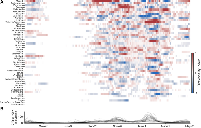
Dynamics of the COVID19 pandemic in Spain. Panel A shows the average normalized directionality index (\(DI_i\)) for each province, reflecting the net information flow during the pandemic. Provinces are sorted by their total \(DI_i\) values. Transfer entropy (\(TE_{i \rightarrow j}\)) was computed using a sliding window of \(\omega = 28\) days, with a step size of \(\delta = 7\) days, and embedding dimension \(q = 1\). Panel B shows the number of daily reported COVID19 cases per 100,000 inhabitants over the same period, with each curve representing a different province. See Supplementary Fig. S14 for individual time series by province.
The results indicate that Madrid was the primary driver of COVID19 cases throughout the pandemic, followed by Álava and Zaragoza (Fig. 5A). Conversely, the Canary and Balearic Islands, along with Soria, were among the most influenced regions. This is expected, as the islands’ isolation reduces their likelihood of being significant drivers, and Soria is Spain’s least populated province. Notably, among the top three driver regions, Zaragoza appears as a key province connecting Barcelona and Madrid, and it played a crucial role as a driver during the second wave, which we will discuss further in this section. The results also show that, although Madrid was the main driver overall, its role shifted between pandemic waves (Fig. 5A and B). During the second wave, Madrid acted as a strong driver, whereas in the third wave, it was more of a driven region. This aligns with Spain’s seasonal mobility patterns, where many people travel out of Madrid during the summer and return during the Christmas season.
Focusing on the beginning of the pandemic, our analysis identifies Álava, along with Madrid, as one of the main drivers of COVID19 spread in Spain. This finding aligns closely with the early pandemic timeline in the country58. As reported by El País, a significant superspreading event occurred in late February 2020, when a funeral held in Vitoria (the capital of Álava) became the largest recorded outbreak at that time. More than 60 attendees at the ceremony were infected, marking a major early milestone in the spread of the virus in Spain59.
Given the likely influence of population movement at the onset of the second COVID19 wave in Spain, we decided to analyze this period in greater detail. At the beginning of Summer, our results show that Lleida started acting as an important driver, probably driving an outbreak of cases in Zaragoza, through Huesca, and later in Madrid. This event is known to have happened due to the arrival of seasonal workers who went to Lleida and Huesca and then got back to Zaragoza and Madrid60. In Fig. 5B, the peak of cases observed in July corresponds to Lleida61. The spreading pattern of this event can be seen in Fig. 6, which shows all Spanish provinces coloured by daily COVID19 incidence and the significant net flow of information \(DI^+_{i \rightarrow j}\) between them. Our results showed how the local \(TE_{i \rightarrow j}(t)\) can help uncover spatio-temporal spreading patterns of an epidemic process such as the COVID19 pandemic.
Fig. 6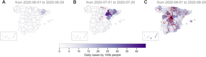
Transfer of entropy between Spanish provinces during the Summer. The maps show Spanish provinces coloured by the number of daily COVID19 cases by 100k inhabitants. Red arrows indicate the net flow of information \(DI^+_{i \rightarrow j}\) between provinces during 28 days starting at different dates. The base map was retrieved from CNIG https://centrodedescargas.cnig.es/CentroDescargas/ under CC-BY 4.0 Licence https://www.ign.es/resources/licencia/Condiciones_licenciaUso_IGN.pdf.
Evaluating the impact of non-pharmaceutical interventions: the case of closing bars in Catalunya
In previous work, we analyzed the policy’s impact on population mobility and observed a significant reduction in movements during this period, unlike Madrid, which served as a control case where no such policy was applied. Moreover, the reduction in mobility in Catalunya was found to correlate significantly with a decrease in new infections4. In this section, we extended our analysis using the mobility-based TE framework to study the relationship between mobility and the rate of new cases, leveraging population mobility and COVID19 case data reported at a finer spatial resolution (see Materials and Methods). Specifically, TE was calculated at the Basic Health Areas (BHAs) level for Catalunya and Madrid. We first examined the effects of using this higher spatial resolution on previously observed patterns of mobility and disease spread. Subsequently, we applied the mobility-based TE framework to evaluate the specific impact of the policy.
In a previous section (Measuring Information Flow Between Mobility Patterns and Epidemic Spread), we demonstrated a significant negative correlation between Transfer Entropy (TE) and geographic distance across pairs of provinces (see Supplementary Fig. S8). In contrast, at the Basic Health Area (BHA) level, while the total number of trips still exhibits a significant negative correlation with distance for both Catalunya and Madrid, the relationship between TE (or ETE) and geographic distance does not show a significant correlation (see Supplementary Figs. S15 and S16). One possible explanation for this discrepancy is that intra-province movement faced fewer restrictions during the pandemic, as such mobility was primarily work-related. In contrast, inter-province movement was more often associated with leisure. Additionally, we analyzed the relationship between the average values of dynamic TE/ETE over time and global TE/ETE in Catalunya and Madrid. We find significant correlations for both cases (see Supplementary Figs. S17 and S18), in agreement with the results observed at the province level (see Supplementary Fig. S12).
In the following, we analyzed the dynamic patterns \(R_{ij}(t)\) and \({\hat{C}}_{j}(t)\) around the time when the policy of closing bars and restaurants was applied in Catalunya. Two weeks after the application of the policy in Catalunya, the daily incidence \({\hat{C}}(t)\) and the mobility M(t) for this region changed their trends and started decreasing (see Supplementary Fig. S19A and B). We also calculated the rate of change for the daily incidence and found that a week after the policy was applied, there was an abrupt deceleration in the rate of change of new cases in Catalunya, whereas in Madrid, there were no changes (see Supplementary Fig. S19C). We calculate the correlation between mobility and the rate of change for the daily incidence in Catalunya and Madrid, for the whole of 2020 (Fig. 7A-B), and for the period when the policy was applied in Catalunya (Fig. 7C-D). The results showed a moderate correlation when the whole year was considered with \(R=0.25\) and \(R=0.14\) for Catalunya and Madrid, respectively (Fig. 7A-B). However, when the correlation is calculated throughout the policy we found a very strong correlation between mobility and the rate of change for the daily incidence with an \(R=0.84\) for Catalunya (\(p=5e-11\)), while for Madrid the correlation was close to zero and statistically not significant (Fig. 7C-D).
Fig. 7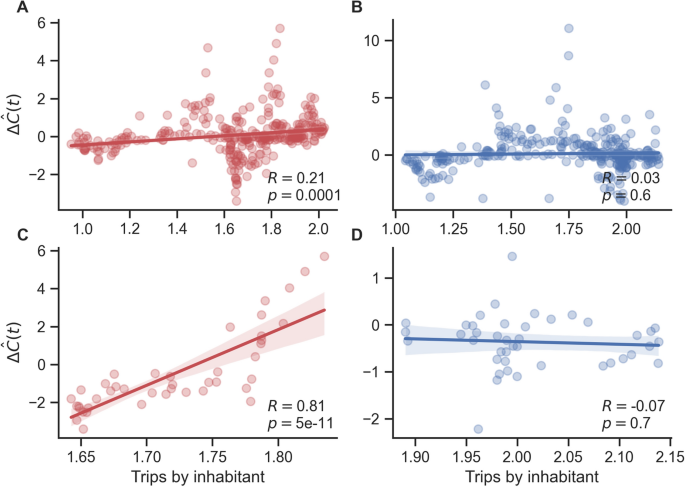
Correlations between the number of trips M(t) per inhabitant and the rate of change of \(\Delta \hat{C}_i(t)\). Panels A and B show the relations between the number of trips M(t) per inhabitant and the rate of change of daily reported new cases \(\Delta \hat{C}_i(t)\) for Catalunya and Madrid, respectively, considering the period between March 2020-03-01 and 2021-02-01. Panels C and D show the relations between the number of trips M(t) per inhabitant and the rate of change of \(\Delta{\hat{C}}_j(t)\) for Catalunya and Madrid respectively, considering the period in which the policy of closing bars and restaurants was applied in Catalunya; the period of the application of the policy spanned between 2020-10-16 and 2020-11-26. The rate of change of \(\Delta {\hat{C}}_i(t)\) was calculated using a first-order finite difference approximation.
Finally, we analyzed the \(ETE_{ij}(t)\) patterns in Catalunya during the period around the NPI application. As shown in Fig. 8, when the policy was implemented, the average values of both \(R_{ij}(t)\) and \({\hat{C}}_j(t)\) were rising in Catalunya, indicating there was a COVID19 outbreak starting in different BHAs. In contrast, Madrid had already experienced a recent outbreak \(R_{ij}(t)\), and \({\hat{C}}_j(t)\) were gradually declining. In both regions, it could be hypothesized that a reduction in \(R_{ij}(t)\) might cause a subsequent decrease in \({\hat{C}}_j(t)\), potentially leading to an increase in \(ETE_{ij}(t)\). However, a significant increase in the average \(ETE_{ij}(t)\) was only observed for Catalunya. This suggests that during the NPI period, the reduction in mobility, reflected by a decrease in \(R_{ij}(t)\), could be causally linked to the observed decline in \({\hat{C}}_j(t)\) in many BHAs. In Madrid, by contrast, no significant increase in the average \(ETE_{ij}(t)\) was detected, indicating that the decline in \({\hat{C}}_j(t)\) likely preceded the reduction in \(R_{ij}(t)\) and was not directly related, even though the average trends may appear correlated.
Fig. 8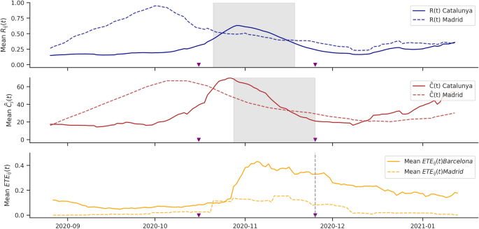
Impact of the temporary closure of bars and restaurants in Catalunya. The panel shows the evolution over time of the mobility-associated risk \(R_{ij}(t)\), the number of new COVID19 cases per 100,000 inhabitants \({\hat{C}}_j(t)\), and the effective transfer entropy \(ETE_{ij}(t)\), all averaged over the basic health areas of Madrid and Catalunya. Purple arrows indicate the start and end dates of the bar and restaurant closure policy in Catalunya (October 16 to November 25, 2020). The grey shaded area represents the sliding window used to compute \(TE_{ij}(t)\) and the \(ETE_{ij}(t)\) at the end of the intervention period.
A closer examination of the dynamic ETE patterns among BHAs during this period reveals notable shifts in areas on the outskirts of Barcelona. The results also showed that many BHAs in the sanitary regions in the outskirts of Barcelona began exhibiting information transfer during a time that coincided with a decline in the number of new COVID19 cases across several areas (see Supplementary Fig. S20). This aligns with the patterns observed in Fig. 8, suggesting a temporal association between reduced mobility and the observed decrease in case numbers during the NPI period in Catalunya. Taken together, the results discussed in this section demonstrate that dynamic ETE patterns may serve as a useful signal for identifying periods when changes in population mobility were closely associated with shifts in disease transmission dynamics.
Recovering disease spreading patterns with mobility-based transfer entropy.
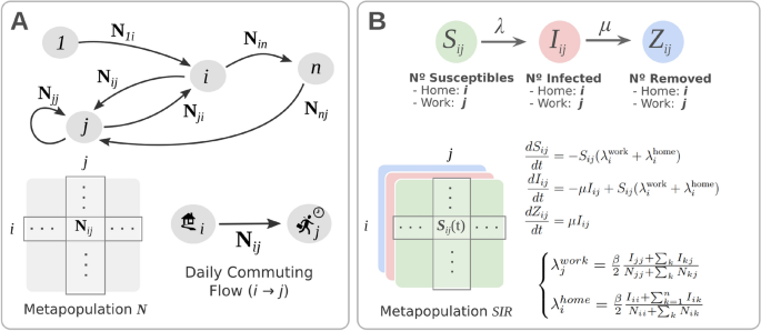
To assess whether our empirical findings could be replicated in a controlled scenario, we simulated an epidemic using a metapopulation SIR model (Fig. 1A-B). Further insight into the simulation approach can be found in Epidemic Simulations. By simulating a simple model, we were able to isolate and examine the mechanisms by which mobility structures shape TE patterns and improve the interpretation of our real-world results. We initiated outbreaks in a single location and evaluated how inter-regional mobility influenced the spread of infection to neighboring areas. We used metapopulation networks of increasing complexity–ranging from a simple linear chain, to a ring, a extended star topology (Supplementary Fig. S21), and finally a model of Spain based on empirical mobility data between provinces.
By focusing on simplified scenarios where the relationship between mobility and transmission dynamics can be explicitly traced, we identified distinct conditions under which significant TE is observed between patches. We present results for the case of the metapopulation model with a extended star-like mobility network previously proposed62, with the initial outbreak seeded in one of the peripheral nodes (Fig. 1A). The epidemic was simulated for 90 days using parameters representative of COVID19: a basic reproduction number \(R_0 = 2.5\) and an average recovery time of \(\mu ^{-1} = 5\) days (see Materials and Methods for details). In this scenario, infections first peak at the origin node and then propagate sequentially to neighboring and downstream nodes (Fig. 1C).
We first analyzed the global effective transfer entropy between each pair of time series \(X_{ij}\) and \(Y_j\), corresponding encoded mobility-associated risk flows from i to j, and the encoded normalized incidence time series of j. Although the underlying mobility network is static, the mobility-associated risk signal \(R_{ij}(t)\) is time-dependent, as it combines fixed commuting flows with dynamically changing infection prevalence. As such, it serves as a meaningful, time-varying proxy for potential exposure between regions, allowing TE to detect dynamic influence patterns even when the contact structure remains fixed. The results show that global ETE patterns qualitatively reproduce the structure of the underlying mobility network (Fig. 9B). However, different values of the encoding parameter q led to different TE signatures. When \(q = 1.0\), we observed frequent back-transfer of entropy from the target to the source patches. This effect reflects the synchronous timing of infection events across regions in the model, which assumes instantaneous infection and reporting. Since the delay \(\delta\) between infection and case count is only one day, many regions become synchronized, resulting in reciprocal TE. In contrast, using \(q = 0.5\) mitigated this back-transfer effect (Supplementary Fig. S25 and S26). With a lower q, the initial rise in \(R_{ij}\) preceded the increase in \({\hat{C}}_j\) by a greater margin, more closely capturing the signal between mobility-associated risk and cases. As such, we selected \(q = 0.5\) for the subsequent TE analyses, as it yielded results more consistent with the mechanistic transmission pathways.
To evaluate the effect of the mobility on the spreading between regions, we measured the dynamic effective transfer entropy \(ETE_{i \rightarrow j}(t)\) between every pair of regions without considering the mobility as we did with the real datasets (see Measuring Information Flow Between Mobility Patterns and Epidemic Spread). For each scenario, we calculated the effective TE using the parameters \(\omega =28\) days, \(\delta =1\) days, and \(q=0.5\). We compared the networks of information flow obtained accounting and without accounting for mobility. We found that when the effective TE is measured considering the mobility, the influence network recovers the structure of the metapopulation through which the epidemic spreads (Fig. 9D). However, if the effective \(TE_{i \rightarrow j}\) is measured only considering the time-series of cases, the network of influences contains many indirect influences (Supplementary Fig. S22). For instance, on day 36, we can observe that the network of influences inferred without considering mobility shows that regions M3 and M9 influence distant regions M8 and M4, respectively, which are not connected through the mobility network. On the contrary, when the effective \(TE_{i \rightarrow j}\) is measured considering the cases at the source region together with the mobility patterns, we can see how the influence network changes but is always constrained by the structure of the metapopulation. These results are in agreement with those found when analysing the information flow using real data for Spain (see section Measuring Information Flow Between Mobility Patterns and Epidemic Spread). Furthermore, similar results were found for other commuting network structures, including the simple chain and the ring (see Supplementary Fig. S23 and S24). Hence, these results show that if mobility is not considered, the TE measures information flow between regions that are not connected through daily commuters, indicating spurious interactions.
Fig. 9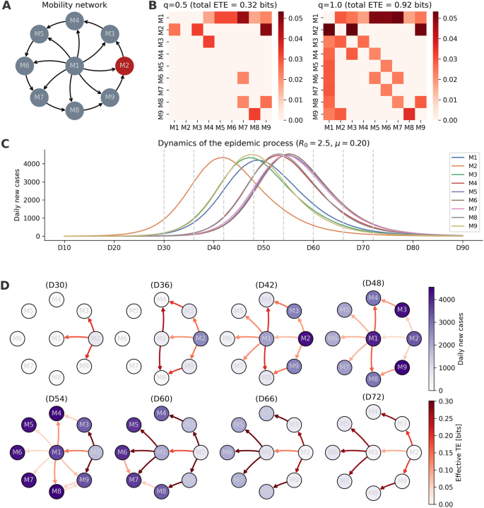
Application of Transfer Entropy to infer a causal relationship between population mobility and the spread of an epidemic in a metapopulation SIR model. Panel A shows the structure of the commuting network, each node has a population of 100, 000 inhabitants, and the number of daily commuters is 5000 in each arrow. Panel B shows the global ETE between each pair of nodes for two different values of the embedding parameter, \(q=0.5\) and \(q=1.0\). Panel C shows the average over 1, 000 simulations of the normalized number of cases as a function of time (in days) obtained using an infection rate \(R_0=2.5\) and a recovery rate \(\mu ^{-1}=5\). Panel D shows the net value of \(ETE_{i \rightarrow j}\) transferred at different days throughout the epidemic and the number of daily new cases in each node. The selected days shown in D are indicated in C as dashed gray lines. ETE parameters \(\delta =1\) days, \(\omega =28\) days and \(q=0.5\) were used. The red node in A is the region where the epidemic started, and the initial number of infected individuals was set to \(I_0=3\).
Figure 9D illustrates two distinct scenarios where dynamic entropy transfer between patches is evident. At the beginning of the epidemic, an increase in risk in M2 precedes and likely signals subsequent rises in cases within M1, M3, and M9, highlighting an entropy transfer originating from M2 around D30. Later, around D54, a different pattern emerges: a decrease in risk in M2 appears to anticipate similar declines in other patches, showing another instance of entropy transfer from M2 to M1, M3, and M9. These results show the adaptability of the dynamic ETE, which responds to various epidemic phases, revealing a complex and evolving influence network (Fig. 9C and D).
We also conducted a SIR-based simulation using real population data and inter-province mobility matrices from Spain during the COVID19 pandemic. Because the SIR model does not incorporate dynamic mobility, we considered two static scenarios: one representing pre-lockdown conditions and the other post-lockdown. We calculated both the dynamic and the global ETE and DI between the provinces as described in Epidemic Simulations in the Material and Methods. The results show a marked decline in total global ETE in the lockdown scenario compared to the pre-lockdown case (see Supplementary Fig. S27), indicating a significant reduction in inter-provincial information flow due to restricted mobility. In addition to this overall decrease, we observed notable shifts in the roles of specific provinces. For example, Zaragoza and Toledo exhibited a substantial drop in incoming ETE during the lockdown, whereas others, like Burgos, became more prominent receivers of information flow. These changes are mirrored in the patterns of dynamic DI over time (Supplementary Figs. S28 and S29), highlighting how mobility restrictions reshaped the epidemic influence network. Altogether, these findings reinforce the relevance of mobility data in uncovering potential causal pathways of epidemic spread and emphasize the value of dynamic information-theoretic measures in characterizing evolving transmission dynamics.
We also examined the relationship between inter-provincial distances and \(TE_{i \rightarrow j}\) in both the pre-lockdown and lockdown scenarios. A significant negative correlation was observed in both cases–\(R = -0.19\) (\(p = 10^{-7}\)) pre-lockdown and \(R = -0.18\) (\(p = 10^{-5}\)) during lockdown–indicating that transfer entropy tends to decrease with increasing distance between provinces (Supplementary Fig. S30A and B). These findings are consistent with those obtained from the real-world data (Supplementary Fig. S8). To test whether this spatial dependency arises from mobility structure or is an artifact of the simulation, we conducted additional experiments under a homogeneous mixing assumption. In these simulations, all outgoing trips from each province were redistributed uniformly across other regions, thereby removing the natural correlation between mobility and geographic distance. Under this setup, the correlation between inter-provincial distances and \(TE_{i \rightarrow j}\) became statistically non-significant (Supplementary Fig. S30C), supporting the idea that the spatial pattern of information flow is driven by structured mobility patterns rather than random mixing.
Finally, we compared the global ETE values obtained from real-world data with those derived from simulations. The overall Pearson correlation was \(R = 0.255\) with a highly significant p-value of \(10^{-38}\) (Supplementary Fig. S31). While modest, this correlation reflects the fundamental differences between simulated and real epidemic dynamics. In the simulations, mobility is static, and each province experiences only a single epidemic wave. In contrast, the real-world epidemic involves dynamic changes in mobility and multiple waves of transmission. Despite these simplifications, the simulations capture essential features of the observed TE patterns, providing valuable insights into the mechanisms underlying epidemic spread. Taken together, these results confirm that the observed TE signals are not merely statistical artifacts of noisy real-world data, but can mechanistically arise from structured, mobility-driven transmission processes. The use of synthetic outbreaks enabled us to isolate and scrutinize the causal pathways of epidemic spread, demonstrating how TE can capture influence patterns aligned with known transmission routes. By comparing networks with and without incorporating mobility data, we identified the conditions under which spurious or indirect interactions may appear. This reinforces the validity of our methodological framework and highlights the value of mobility-informed TE analysis in detecting meaningful, time-resolved influence patterns in epidemic dynamics.