Brain-wide representations of prior information in mouse decision-making

For the Ephys data, we used the 2024 IBL public data release51, which is organized and shared using a modular architecture described previously52. It comprises 699 recordings from Neuropixels 1.0 probes. One or two probe insertions were realized over 459 sessions of the task, performed by a total of 139 mice. For a detailed account of the surgical methods for the headbar implants, see appendix 1 of ref. 33. For a detailed list of experimental materials and installation instructions, see appendix 1 of ref. 35. For a detailed protocol on animal training, see the methods of refs. 33,35. For details on the craniotomy surgery, see appendix 3 of ref. 35. For full details on the probe tracking and alignment procedure, see appendices 5 and 6 of ref. 35. The spike sorting pipeline used by IBL is described in detail in ref. 35. For the WFI data, we used another dataset consisting of 52 recordings of the dorsal cortex, realized over 52 sessions of the task, performed by a total of 6 mice. A detailed account of the WFI data acquisition and preprocessing was reported previously53.

All experimental procedures involving animals were conducted in accordance with local laws and approved by the relevant institutional ethics committees. Approvals were granted by the Animal Welfare Ethical Review Body of University College London, under licences P1DB285D8, PCC4A4ECE and PD867676F, issued by the UK Home Office. Experiments conducted at Princeton University were approved under licence 1876-20 by the Institutional Animal Care and Use Committee (IACUC). At Cold Spring Harbor Laboratory, approvals were granted under licences 1411117 and 19.5 by the IACUC. The University of California at Los Angeles granted approval through IACUC licence 2020-121-TR-001. Additional approvals were obtained from the University Animal Welfare Committee of New York University (licence 18-1502); the IACUC at the University of Washington (licence 4461-01); the IACUC at the University of California, Berkeley (licence AUP-2016-06-8860-1); and the Portuguese Veterinary General Board (DGAV) for experiments conducted at the Champalimaud Foundation (licence 0421/0000/0000/2019).

Mice

Animals were housed under a 12 h−12 h light–dark cycle—either normal or inverted, depending on the laboratory—and had unrestricted access to food and water except on training days. Depending on the laboratory, electrophysiology recordings and behavioural training took place during either the light or dark phase of the cycle. In total, data were collected from 139 adult C57BL/6 mice (94 male, 45 female), purchased from Jackson Laboratory or Charles River. On the day of electrophysiological recording, these mice ranged in age from 13 to 178 weeks (mean, 44.96 weeks; median, 27.0 weeks) and weighed between 16.1 and 35.7 g (mean 23.9 g, median 23.84 g).

Inclusion criteria for the analysisCriteria for trial inclusion

All trials were included except when the animals did not respond to the stimulus (no movement, no response) or when the first wheel movement time (reaction time) was shorter than 80 ms or longer than 2 s.

Criteria for session inclusion

All sessions were included except sessions with fewer than 250 trials (counting only included trials). In total, 41 sessions in Ephys and 1 session in WFI did not meet the criteria for the minimum number of trials.

Criteria for neural recording inclusion

An insertion was included in the analysis if it had been resolved, that is, if histology clearly revealed the path of the probe throughout the brain, as defined previously35. A neuron, identified during the spike sorting process, was included if it passed three quality control (QC) criteria (amplitude > 50 μV; noise cut-off 

For the region-level analysis, after applying these criteria, we were left with 414 sessions for the Ephys dataset. Initially, we considered 418 (459 − 41) sessions that had more than 250 included trials, but 4 of these did not have any recorded regions meeting the minimum number of units required. Our region-level analysis spans 242 brain regions, defined by the Allen Common Coordinate Framework31, recorded by at least one included insertion. Our Ephys region-level analysis spans 2,289 region–sessions, which are aggregated across sessions to give results at the region level. For the WFI dataset, we were left with 51 (52 − 1) sessions that had more than 250 included trials. They all had at least one recorded region meeting the minimum number of recorded pixels required. The imaging spans 32 regions of the dorsal cortex—which are included among the 242 regions decoded in the Ephys analysis, for a total of 1,539 ((51 × 32) − 28 − 65) region–sessions. This total accounts for the fact that not every region was visible in all sessions, summing to 28 non-observed region–sessions. Moreover, 65 region–sessions were excluded because the regions recorded had fewer than 5 pixels.

For the session-level analysis, neurons along the probes were used and most of the sessions in Ephys (457 out of 459) had at least 5 recorded units that passed the QC. Taking into account the session inclusion criteria, session-level analysis was performed on 416 sessions. All of the 51 WFI sessions passed the minimal number of trials criteria and were therefore included in the analysis.

Criteria for the embodiment analysis

Only sessions with available DLC features could be used for the embodiment prior analysis, which requires access to body position. For the Ephys dataset, we analysed the 171 sessions (out of 459) for which the DLC features met the quality criteria defined previously35, and for which the other inclusion criteria were met. This resulted in a total of 806 region–sessions. WFI sessions were excluded from this analysis as no video recordings were available.

Criteria for the eye position analysis

Reliable tracking of eye position from video recordings was not possible for some sessions due to video quality issues. Thus, we recovered reliable eye position signals from 44 out of the 53 of sessions in which we had recorded from either VISp or LGd, the two regions for which we specifically analysed the impact of eye position.

Joint decoding of DLC features and eye position signals

We performed the joint decoding of DLC features and eye position signals on the 124 sessions in which the DLC features met the QC criteria and also in which the eye position signals were reliable, for a total of 660 region–sessions.

Difference compared with the Brain Wide Map inclusion criteria

There were two key differences between our inclusion criteria and those used in the Brainwide Map32. First, the Brainwide Map included only regions that had at least two recording sessions, whereas we included regions irrespective of the number of recording sessions. Second, we excluded sessions that had fewer than 250 trials after applying trial inclusion criteria, a criterion not applied in the Brainwide Map.

Electrophysiology data

Spike counts were obtained by summing the spikes across the decoding window for each neuron and included trial. If there were U units and T trials, this binning procedure resulted in a matrix of size U × T. For the ITI, the time window for the main decoding was (−600 ms,−100 ms) relative to stimulus onset and, for the post-stimulus window, it was (0 ms, +100 ms) relative to stimulus onset. We used L1-regularized linear regression to decode the Bayes-optimal prior from the binned spike count data using the scikit-learn function sklearn.linear_model.Lasso (using one regularization parameter). We used L1 for Ephys because it is more robust to outliers, which are more likely to occur in single-cell recordings, notably because of drift. The Bayes-optimal prior was inferred from the sequence of stimuli for each session (see the ‘Behavioural models’ section and the Supplementary Information). This decoding procedure yielded a continuous-valued vector of length T.

WFI data

For the WFI data, we used L2-regularized regression as implemented by the scikit-learn function sklearn.linear_model.Ridge (one regularization parameter). We used L2 regularization instead of L1 for WFI data because L2 tends to be more robust to collinear features, which is the case across WFI pixels. We decoded the activity from the vector of the region’s pixels for a specific frame of the data. The activity is the change in fluorescence intensity relative to the resting fluorescence intensity ΔF/F. Data were acquired at 15 Hz. Frame 0 corresponds to the frame containing stimulus onset. For the ITI, we used frame −2 relative to the stimulus onset. This frame corresponds to a time window of which the start ranges from −198 to −132 ms before the stimulus onset, and of which the end ranges from −132 to −66 ms, depending on the timing of the last frame before stimulus onset. For the post-stimulus interval, we used frame +2, which corresponds to a time window of which the start ranges from 66 to 132 ms from stimulus onset, and extends to 132 to 198 ms after onset. This interval is dependent on the timing of the first frame after stimulus onset, which can occur at anytime between 0 and 66 ms after onset. If there are P pixels and T trials, this selection procedure results in a matrix of size P × T.

Reversal curves

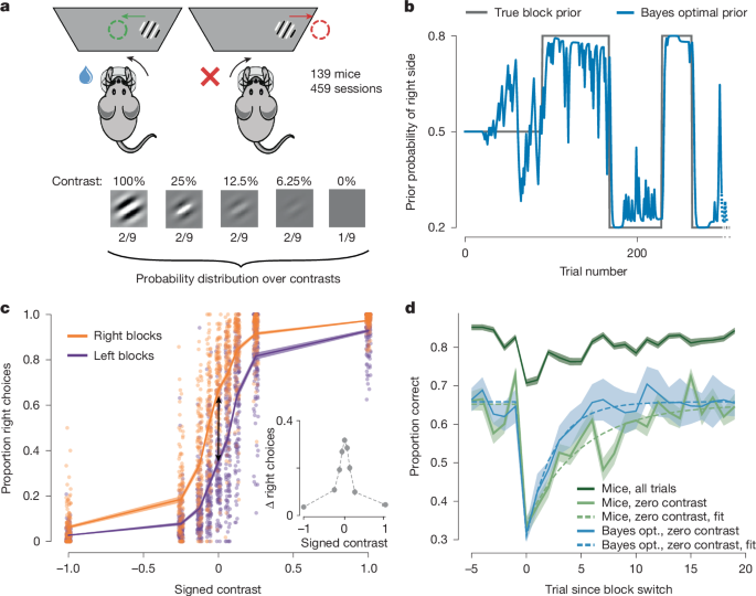
To analyse mouse behaviour around block reversals, we plotted the reversal curves defined as the proportion of correct choices as a function of trials, aligned to a block change (Fig. 1d). These were obtained by computing one reversal curve per mouse (pooling over sessions) and then averaging and computing the s.e.m. across the mouse-level reversal curves. For comparison purposes, we also showed the reversal curves for the Bayes-optimal model with a probability-matching decision policy. We did not plot s.e.m. values but instead s.d. values in this case as there was no variability across agents to account for.

To assess the differences between the mouse behaviour and the agent that samples actions from the Bayes-optimal prior, we fitted the following parametric function to the reversal curves:

$$p({\rm{correct}}\;{\rm{at}}\;{\rm{trial}}\,t)=(B+(A-B)\times {{\rm{e}}}^{-t/\tau })\times (t\ge 0)+B\times (t

with t = 0 corresponding to the trial of the block reversal, τ the decay constant, B the asymptotic performance and A the drop in performance right after a block change.

We fitted this curve using only zero-contrast trials, between the 5 pre-reversal trials and the 20 post-reversal trials. We restricted our analysis to the zero-contrast trials to focus on trials in which mice could only rely on block information to decide. This implied that we only used a small fraction of the data. To be precise, across the 459 sessions, we had an average of 10 reversals per session, and the proportion of zero-contrast trials is 11.1%. Fitting only on the zero-contrast trials around reversals led us to use around 28 trials per session, which accounts for around 3% of the behavioural data—when excluding the first 90 unbiased trials, the average session consists of 555 trials.

To make up for this limited amount of data, we used a jackknifing procedure for fitting the parameters. The procedure involved iteratively leaving out one mouse and fitting the parameters on the N − 1 = 138 zero-contrast reversal curves of the held-in mice. The results of the jackknifing procedure are shown in Extended Data Fig. 1.

Nested cross-validation procedure

Decoding was performed using cross-validated, maximum-likelihood regression. We used the scikit-learn Python package to perform the regression53, and implemented a nested cross-validation procedure to fit the regularization coefficient.

The regularization coefficient was determined by two nested fivefold cross-validation schemes (outer and inner). We first described the procedure for the Ephys data. In the outer cross-validation scheme, each fold was based on a training/validation set comprising 80% of the trials and a test set of the remaining 20% (random interleaved trial selection). The training/validation set was itself split into five sub-folds (inner cross-validation) using an interleaved 80–20% partition. Cross-validated regression was performed on this 80% training/validation set using a range of regularization weights, chosen for each type of dataset so that the bounds of the hyperparameter range are not reached. For each modality, we searched a logarithmically spaced grid of ridge-regularization weights that was tuned to the dimensionality of the corresponding feature space: for Ephys, the grid was C ∈ {10−5, 10−4, 10−3, 10−2, 10−1}; for WFI, C ∈ {10−5, 10−4, 10−3, 10−2}; for the set of DLC-extracted behavioural features, C ∈ {10−4, 10−3, 10−2, 10−1, 1, 10, 100}; for eye-position features, C ∈ {10−4, 10−3, 10−2, 10−1, 1, 10, 100, 1,000, 10,000}; for the combined DLC-features + eye-position model, the same broad grid C ∈ {10−4, 10−3, 10−2, 10−1, 1, 10, 100, 1,000, 10,000} was used; for the Ephys-based neurometric decoder, C ∈ {10−5, 10−4, 10−3, 10−2, 10−1, 1}; and for the widefield neurometric decoder, C ∈ {10−5, 10−4, 10−3, 10−2}.

The regularization weight selected with the inner cross-validation procedure on the training/validation set was then used to predict the target variable on the 20% of trials in the held-out test set. We repeated this procedure for each of the five ‘outer’ folds, each time holding out a different 20% of test trials such that, after the five repetitions, 100% of trials have a held-out decoding prediction. For WFI, the procedure was very similar but we increased the number of outer folds to 50 and performed a leave-one-trial-out procedure for the inner cross-validation (using the efficient RidgeCV native sklearn function). We did this because the number of features in WFI (number of pixels) is much larger than in Ephys (number of units): around 167 units on average in Ephys when decoding on a session-level from both probes after applying all quality criteria, versus around 2,030 pixels on a session-level in WFI when decoding from the whole brain.

Furthermore, to average out the randomness in the outer randomization, we ran this procedure ten times. Each run used a different random seed for selecting the interleaved train/validation/test splits. We then reported the median decoding score R2 across all runs. Regarding the decoded prior, we took the average of the predicted priors (estimated on the held-out test sets) across the ten runs.

Assessing statistical significance

Decoding a slow varying signal such as the Bayes-optimal prior from neural activity can easily lead to false-positive results even when properly cross-validated. For example, slow drift in the recordings can lead to spurious, yet significant, decoding of the prior if the drift is partially correlated with the block structure34,54. To control for this problem, we generated a null distribution of R2 values and determined significance with respect to that null distribution. This pseudosession method is described in detail previously34.

We denote \(X\in {{\mathbb{R}}}^{N\times U}\) the aggregated neural activity for a session and \(Y\in {{\mathbb{R}}}^{N}\) the Bayes-optimal prior. Here, N is the number of trials and U the number of units. We generated the null distribution from pseudosessions, that is, sessions in which the true block and stimuli were resampled from the same generative process as the one used for the mice. This ensures that the time series of trials in each pseudosession shares the same summary statistics as the ones used in the experiment. For each true session, we generated M = 1,000 pseudosessions, and used their resampled stimulus sequences to compute Bayes-optimal priors \({Y}_{i}\in {{\mathbb{R}}}^{N}\), with i ∈ [1, M] the pseudosession number. We generated pseudoscores \({R}_{i}^{2}\in {R},{i}\in [1,{M}]\) by running the neural analysis on the pair (X,Yi). The neural activity X is independent of Yi as the mouse did not see Yi but Y. Any predictive power from X to Yi would arise from slow drift in X unrelated to the task itself. These pseudoscores \({R}_{i}^{2}\) were compared to the actual score R2 obtained from the neural analysis on (X,Y) to assess statistical significance.

The actual R2 is deemed to be significant if it is higher than the 95th percentile of the pseudoscores distribution \(\{{R}_{i}^{2},{i}\in [1,{M}]\}\). This test was used to reject the null hypothesis of no correlation between the Bayes optimal prior signal Y and the decoder prediction. We defined the P value of the decoding score as the quantile of R2 relative to the null distribution \(\{{R}_{i}^{2},{i}\in [1,{M}]\}\).

For each region of the brain that we recorded, we obtained a list of decoding P values, where a P value corresponds to the decoding of the region’s unit activity during one session. We used Fisher’s method to combine the session-level P values of a region into a single region-level P value (see the ‘Fisher’s method’ section for more details).

For effect sizes, we computed a corrected R2, defined as the actual score R2 minus the median of the pseudoscores distribution, \(\{{R}_{i}^{2},{i}\in [1,{M}]\}\). The corrected R2 of a region is the mean of the corrected R2 for the corresponding sessions.

Choosing between Pearson and Spearman correlation methods

In our statistical analyses, we prioritized using Spearman’s correlation when datasets included outliers, as it is robust against non-normal distributions. In other cases, we opted for Pearson’s correlation to assess linear relationships. For paired comparisons, we used the Wilcoxon signed-rank test, which likewise makes no assumption of normality while retaining sensitivity to systematic shifts between conditions.

Fisher’s method

Fisher’s method is a statistical technique used to combine independent P values to assess the overall significance. It works by transforming each P value into a χ2 statistic and summing these statistics. Specifically, for a set of P values (one per session given a region), p1, p2, p3, …, Fisher’s method computes the test statistic

$${X}^{2}=-\,2\sum _{i}\mathrm{ln}({p}_{i})$$

This statistic follows a χ2 distribution with 2 × Nsessions d.f., \({\chi }_{2\times {N}_{{\rm{sessions}}}}^{2}\), under the null hypothesis that all individual tests are independent and their null hypotheses are true. If the computed test statistic X2 exceeds a critical value from the χ2 distribution, the combined P value \(p({\chi }_{2\times {N}_{{\rm{sessions}}}}^{2}\ge {X}^{2})\) is considered significant and the null hypothesis is rejected.

Cosmos atlas

We defined a total of ten annotation regions for coarse analyses. Annotations include the major divisions of the brain only: isocortex, olfactory areas, hippocampal formation, cortical subplate, cerebral nuclei, thalamus, hypothalamus, midbrain, hindbrain and cerebellum. A detailed breakdown of the Cosmos atlas is provided in Extended Data Fig. 5.

Granger causality

To understand how prior information flows between brain regions, we performed a Granger causality analysis on the Ephys and WFI data during the ITI.

For each Ephys session, we considered the neural activity from −600 ms to −100 ms before stimulus onset, segmented into 50 ms bins, yielding 10 bins per region. For each bin, we predicted the Bayes-optimal from the neural activity using the native LassoCV sklearn function, with its default regularization candidates. This leads to a decoded Bayes-optimal prior for each region and bin. We next used a Granger causality analysis to explore whether the prior information in some region Granger-causes prior information in other regions. Granger analysis was run with the spectral connectivity Python library from the Eden-Kramer lab (https://github.com/Eden-Kramer-Lab/spectral_connectivity).

Given a directed pair of regions (for example, from ACAd to VISp) within a session, the Granger analysis assigns an amplitude to each frequency in the discrete Fourier transform. We calculate an overall Granger score by session by averaging the amplitudes across frequencies55.

To assess significance of the overall Granger score for a directed pair and session, we build a null distribution by applying our analysis to 1,000 pseudosessions (see the ‘Assessing statistical significance’ section). After decoding these pseudopriors from neural activity for each region and bin, we perform Granger analysis on these decoded pseudopriors. This creates 1,000 pseudo-Granger scores per directed pair and session. Significance is assessed by comparing the actual Granger score against the top 5% of the pseudo scores.

Granger analysis for the WFI data is very similar to that for Ephys. The main differences are the use the last nine frames before stimulus onset as individual bins and the use of the RidgeCV native function from sklearn for the decoding (see the ‘WFI data’ section).

Initially, we investigate whether communication between regions exceeds what might be expected by chance. To assess this, we analyse the percentage of significant directed pairs between two regions that significantly reflect the prior; we find an average of 71.6% in WFI and 35.9% in Ephys across sessions. We then repeat this analysis for each session across 1,000 pseudosessions. Subsequently, we assess whether the average percentage of significant pairs across sessions falls within the top 5% of the average percentages calculated from these pseudo-sessions, which indeed it does (Extended Data Fig. 10a).

Next, we explore whether the flow of prior information involves more loops than would typically occur by chance. Specifically, we assess whether triadic loops (A>B>A) within a session occur more frequently than expected. To evaluate this, we calculate the percentage of instances in which a significant Granger pair results in a loop of size 3 for each session. We find that an average (across sessions) of 37.7% in WFI and 10.8% in Ephys exceed what would be anticipated by chance, confirming a higher prevalence of loops (Fig. 2h and Extended Data Fig. 10b).

To obtain Granger graphs at the region level, we use Fisher’s method to combine the session-level P values of a directed pair. Lastly, to construct the Granger causality graph at the Cosmos level, we further combine the P values from each directed pair using Fisher’s method once again.

Controlling for region size when comparing decoding scores across Ephys and WFI

With WFI data, the activity signal of a region has always the same dimension across sessions, corresponding to the number of pixels. To control for the effect of region size on the region R2, we performed linear regression across 32 recorded regions to predict the decoding R2 from the number of pixels per region. We found a significant correlation between R2 and the size of the regions (Extended Data Fig. 7d; R = 0.82, P = 9.1 × 10−9). To determine whether this accounts for the correlations between Ephys and WFI R2 correlation (Fig. 2d), we subtracted the R2 predicted by region’s size from the WFI R2 and recomputed the correlation between Ephys R2 and these size-corrected WFI R2 (Extended Data Fig. 7f).

Number of recording sessions per region required to reach significance

For each region showing significance in prior decoding, we conducted a subsampling process to see how many recorded sessions were necessary on average to reach significance. A region r is associated with set of Nr sessions in which its activity was recorded. For a particular region, we can randomly subselect N ∈ [1, Nr] sessions from this set and test the significance of the region given only these N prior decodings.

For each significant region and each possible number N, we repeated this procedure 1,000 times, getting a distribution of P values. We report \({p}_{r}^{N}\), the median of the P-value distribution, as a measure of the significance for prior decoding of the region r given that only N recording sessions are available.

For each number of available sessions N, we report the fraction of the total number of significant regions for which the statistic \({p}_{r}^{N}\) is less than 0.05, as a measure of the number of recordings per region required to reach back our obtained significance levels.

Assessing the significance of decoding weights

Let wi be the weight associated with the neuron i—where i ranges from 1 to U, with U the number of units, for the decoding of U neurons’ activity on a particular region–session. We determine whether the weight is significant by comparing it to the distribution of pseudoweights \(\{{\hat{w}}_{i}^{k},{k}\in [1,{M}]\}\) derived from decoding the M = 200 pseudosessions priors based on neural activity on that same region-session.

wi is deemed to be significant if it is higher than the 97.5th percentile of the pseudoweights distribution or lower than the 2.5th percentile.

Proportion of right choices as a function of the decoded prior

To establish a link between the decoded prior, as estimated from the neural activity, and the mouse behaviour, we plotted the proportion of right choices on zero-contrast trials as a function of the decoded Bayes-optimal prior. For each Ephys (or WFI) session, we decoded the Bayes-optimal prior using all neural activity from that session. We focused this analysis on test trials, held-out during training, according to the procedure described in the ‘Nested cross-validation procedure’ section. For Fig. 2e, we then pooled over decoded priors for all sessions, assigned them to deciles and computed the associated proportion of right choices. In other words, we computed the average proportion of right choices on trials in which the decoded prior is part of each decile.

To quantify the significance of this effect at a session level (Extended Data Fig. 8a), we additionally performed a logistic regression predicting the choice (right or left) as a function of the decoded prior. Let j be the session number; we predict the actions on that session \({a}_{t}^{j}\) (with t the trial number) as a function of the decoded prior:

$$p({a}_{t}^{j}={\rm{right}})=1/[1+\exp (-({\mu }^{j}\times {\widehat{Y}}_{t}^{j}+{c}^{j}))]$$

with \({\widehat{Y}}_{t}^{j}\) the cross-validated decoded Bayes-optimal prior, μj the slope (coefficient of the logistic regression associated with the decoded prior) and cj an intercept. The logistic regression fitting was performed using the default sklearn LogisticRegression function, which uses L2 regularization on weights with regularization strength C = 1.

To assess the statistical significance of these slopes, \({\mu }^{j}\), we generated null distributions of slopes over M = 200 pseudosessions (pseudosessions are defined in the ‘Assessing statistical significance’ section). For each pseudosession, we computed the slope of the logistic regression between proportion of correct choices as a function of the decoded pseudo-Bayes-optimal prior. The decoded pseudo-Bayes-optimal prior was obtained by first computing the pseudo-Bayes-optimal prior for each pseudosession, and then using the neural data from the original session to decode this pseudo-Bayes-optimal prior. The percentage of correct choice was more complicated to obtain on pseudosessions because it requires simulating the mice choices as accurately as possible. As we do not have a perfect model of the mouse choices, we had to approximate this step with our best model, that is, the action kernel model. We used the action kernel model fitted to the original behaviour session and simulated it on each pseudosession to obtain the actions on each trial of the pseudosessions.

From the set of decoded pseudo-Bayes-optimal priors and pseudoactions, we obtained M pseudoslopes \({\mu }_{i}^{\,j},{i}=1\ldots M\) using the procedure described above. As the mouse did not experience the pseudosessions or perform the pseudoactions, any positive coefficient \({\mu }_{i}^{j}\) has to be the result of spurious correlations. Formally, to assess significance, we examine whether the mean slope \((\mu =1/J\times {\sum }_{j=1}^{J}{\mu }^{j})\) is within the 5% top percentile of the averaged pseudoslopes: \(\{\,{\mu }_{i};{\mu }_{i}=1/J\times {\sum }_{j=1}^{J}{\mu }_{i}^{j}\); \(i\in [1,M]\}\). Extended Data Fig. 8a shows this set of M averaged pseudoslopes as a histogram. The red vertical dashed line is the average slope μ.

When applying this null-distribution procedure in Ephys and WFI data, we find that the pseudoslopes in Ephys data are much more positive than in WFI data. This is due to the fact that spurious correlations in Ephys data are likely induced by drift in the Neuropixels probes, whereas WFI data barely exhibit any drift.

Neurometric curves

We used the same decoding pipeline described for the Bayes-optimal prior decoding to train a linear decoder of the signed contrast from neural activity in each region, for the ITI [−600, −100] ms and post-stimulus [0, 100] ms intervals. There are 9 different signed contrasts {−1, −0.25, −0.125, −0.0625, 0, 0.0625, 0.125, 0.25, 1} where the left contrasts are negative and the right contrasts are positive. Given a session of T trials, we denote \(\{{s}_{i}{\}}_{i\in [1,T]}\) the sequence of signed contrasts, \(\{{\hat{s}}_{i}{\}}_{i\in [1,T]}\) the cross-validated decoder output given the neural activity X and \(\{{p}_{i}{\}}_{i\in [1,T]}\) the Bayes-optimal prior. We defined two sets of trial indices for each session based on the signed contrast c and the Bayes-optimal prior: \({I}_{c}^{{\rm{low}}}=\{i| ({s}_{i}=c)\,{\rm{and}}\,{p}_{i} and \({I}_{c}^{{\rm{high}}}\,=\,\{i| ({s}_{i}=c)\) and \({p}_{i} > 0.5\}\) corresponding to the trials with signed contrast c and a Bayes-optimal prior lower or higher than 0.5 respectively.

For these sets, we computed the proportions \({P}_{c}^{{\rm{l}}{\rm{o}}{\rm{w}}}={\rm{\#}}\{{\hat{s}}_{i} > 0;\)\(i\in \,{I}_{c}^{{\rm{l}}{\rm{o}}{\rm{w}}}\}/{\rm{\#}}{I}_{c}^{{\rm{l}}{\rm{o}}{\rm{w}}}\) and \({P}_{c}^{{\rm{high}}}=\#\{{\widehat{s}}_{i} > 0\,;i\in \,{I}_{c}^{{\rm{high}}}\}/\#{I}_{c}^{{\rm{high}}}\). These are the proportions of trials decoded as right stimuli conditioned on the Bayes-optimal prior being higher or lower than 0.5. We fitted a low prior curve to \({\{(c,{P}_{c}^{{\rm{low}}})\}}_{c\in \varGamma }\) and a high prior curve to \({\{(c,{P}_{c}^{{\rm{high}}})\}}_{c\in \varGamma }\), which we called neurometric curves. We used an erf() function from 0 to 1 with two lapse rates for the curves fit to obtain the neurometric curve:

$$f(c)=\gamma +(1-\gamma -\lambda )\times ({\rm{erf}}((c-\mu )/\sigma )+1)/2$$

where γ is the low lapse rate, λ is the high lapse rate, μ is the bias (threshold) and σ is the rate of change of performance (slope). Importantly, we assumed some shared parameters between the low-prior curve and the high-prior curve: γ, λ and σ are shared, while the bias μ is free to be different for low and high prior curves. This assumption of shared parameters provides a better fit to the data compared to models with independent parameters for each curve, as evidenced by lower Bayesian information criterion (BIC) scores during both pre-stimulus (ΔBIC = BIC(independent parameters) − BIC(shared parameters) = 6,482 for Ephys, ΔBIC = 822 for WFI) and post-stimulus periods (ΔBIC = 6,435 for Ephys, ΔBIC = 812 for WFI). We used the psychofit toolbox to fit the neurometric curves using maximal-likelihood estimation (https://github.com/cortex-lab/psychofit). Finally, we estimated the vertical displacement of the fitted neurometric curves for the zero contrast fhigh(c = 0) − flow(c = 0), which we refer to as the neurometric shift.

We used the pseudosession method to assess the significance of the neurometric shift, by constructing a neurometric shift null distribution. M = 200 pseudosessions are generated with their signed contrast sequences, which are used as target to linear decoder on the true neural activity. We fitted neurometric curves to the pseudosessions decoder outputs, conditioned on the Bayes-optimal prior inferred from the pseudosessions contrast sequences.

Stimulus side decoding

To compare the representation of prior information across the brain to the representation of stimulus, we used the stimulus side decoding results from our companion paper32. The decoding of the stimulus side was performed using cross-validated logistic regression with L1 regularization, on a time window of [0, 100] ms after stimulus onset. Only regions with at least two recorded sessions were included, a criteria applied in the companion paper32. The bottom panel of Extended Data Fig. 12b is a reproduction from figure 5a of our companion paper32.

Embodiment

Video data from two cameras were used to extract 7 behavioural variables which could potentially be modulated according to the mice’s subjective prior35:

• Paw position (left and right): Euclidean distance of the DLC-tracked paws to a camera frame corner, computed separately for the right and left paw.

• Nose position: horizontal position of the DLC-tracked nose captured by the left camera.

• Wheeling: wheel speed, obtained by interpolating the wheel position at 5 Hz and taking the derivative of this signal.

• Licking: the left and right edges of the tongue are DLC-tracked with both lateral cameras. A lick is defined to have occurred in a frame if the difference for either coordinate to the subsequent frame is larger than 0.25 times the s.d. of the difference of this coordinate across the whole session. The licking signal is defined as the number of licking events during each time bin of 0.02 s.

• Whisking (left and right): motion energy of the whisker-pad area in the camera view, quantified as the mean across pixels of the absolute grey-scale difference between adjacent frames; computed separately for the left- and right-side cameras.

If we are able to significantly decode the Bayes-optimal prior from these behavioural variables during the [−600 ms, −100 ms] ITI, we say that the subject embodies the prior. For the decoding, we used L1-regularized maximum-likelihood regression with the same cross-validation scheme used for neural data (see the ‘Nested cross-validation procedure’ section). Sessions and trials are subject to the same QC as for the neural data, so that we decode the same sessions and the same trials as the Ephys session-level decoding. For each trial, the decoder input is the average over the ITI [−600, −100] ms of the behavioural variables. For a session of T trials, the decoder input is a matrix of size T × 7 and the target is the Bayes-optimal prior. We use the pseudosession method to assess the significance of the DLC features decoding score R2. To investigate the embodiment of the Bayes-optimal prior signal, we compared session-level decoding of the prior signal from DLC regressors to region–session-level decoding of the prior signal from the neural activity of each region during the session.

DLC residual analysis

The DLC prior residual signal is the part of the prior signal which was not explained away by the DLC decoding, defined as the prior signal minus the prediction of the DLC decoding. We decoded this DLC prior residual signal from the neural activity, using the same linear decoding schemes as previously described.

Eye position decoding

Video data from the left camera were used to extract the eye position variable, a 2D signal corresponding to the position of the centre of the mouse pupil relative to the video border. The camera as well as the mouse’s head were fixed. DeepLabCut was not able to achieve sufficiently reliable tracking of the pupils; we therefore used a different pose-estimation algorithm56, trained on the same labelled dataset used to train DeepLabCut. For the decoding, we used L2-regularized maximum-likelihood regression with the same cross-validation scheme used for neural data, during the [−600 ms, −100 ms] ITI.

The eye-position prior residual signal is the part of the prior signal which is not explained away by the eye position decoding, defined as the prior signal minus the prediction of the eye position decoding. We decode this eye position prior residual signal from the neural activity of early visual areas (LGd and VISp) using the same linear decoding schemes as previously described.

Contribution of DLC and eye-position features to prior embodiment: feature importance

To assess the contribution of DLC and eye position features to prior embodiment, we performed a leave-one-out decoding procedure of the DLC + eye position features. There are five different types of DLC features: licking, wheeling, nose position, whisking and paws positions. Moreover, with the x and y coordinates of the eye position, we had a total of seven types of variables for which we individually performed a separate leave-one-out decoding analysis. The difference between the full decoding R2 and the leave-one-out decoding R2 is a measure of the importance of the knocked-out variable in the full decoding.

Behavioural models

To determine the behavioural strategies used by the mice, we developed several behavioural models and used Bayesian model comparison to identify the one that fits best. We considered three types of behavioural models that differ as to how the integration across trials is performed (how the subjective prior probability that the stimulus will be on the right side is estimated based on history). Within a trial, all models compute a posterior distribution by taking the product of a prior and a likelihood function (the probability of the noisy contrast given the stimulus side; Supplementary information).

Among the three types of models of the prior, the first, called the Bayes-optimal model, assumes knowledge of the generative process of the blocks. Block lengths are sampled as follows:

$$p({l}_{k}=N)\propto \exp (-N/\tau )\times {\mathbb{1}}[20\le N\le 100]$$

with lk the length of block k and \({\mathbb{1}}\) the indicator function. Block lengths are therefore sampled from an exponential distribution with parameter τ = 60 and constrained to be between 20 and 100 trials. When block k − 1 comes to an end, the next block bk, with length lk, is defined as a right block (where the stimulus is likely to appear more frequently on the right) if block bk−1 was a left block (where the stimulus was likely to appear more frequently on the left) and conversely. During left blocks, the stimulus is on the left side with probability γ = 0.8 (and similarly for right blocks). Defining st as the side on which the stimulus appears on trial t, the Bayes-optimal prior probability the stimulus will appear on the right at trial t, \(p({s}_{t}\,|\,{s}_{1:(t-1)})\) is obtained through a likelihood recursion57.

The second model of the subjective prior, called the stimulus kernel model58, assumes that the prior is estimated by integrating previous stimuli with an exponentially decaying kernel. Defining st−1 as the stimulus side on trial t – 1, the prior probability that the stimulus will appear on the right πt is updated as follows:

$${\pi }_{t}=(1-\alpha )\times {\pi }_{t-1}+\alpha \times {\mathbb{1}}[{s}_{t-1}={\rm{right}}]$$

with πt−1 the prior at trial t − 1 and α the learning rate. The learning rate governs the speed of integration: the closer α is to 1, the more weight is given to recent stimuli st−1.

The third model of the subjective prior, called the action kernel model, is similar to the stimulus kernel model but assumes an integration over previous chosen actions with, again, an exponentially decaying kernel. Defining at−1 as the action at trial t − 1, the prior probability that the stimulus will appear on the right πt is updated as follows:

$${\pi }_{t}=(1-\alpha )\times {\pi }_{t-1}+\alpha \times {\mathbb{1}}[{a}_{t-1}={\rm{right}}]$$

For the Bayes-optimal and stimulus kernel models, we additionally assume the possibility of capturing a simple autocorrelation between choices with immediate or multistep repetition biases or choice- and outcome-dependent learning rate40,59. Further details on model derivations are provided in the Supplementary Information.

Model comparison

To perform model comparison, we implemented a session-level Bayesian cross-validation procedure. In this procedure, for each mouse with multiple sessions, we held out one session i and fitted the model on the held-in sessions. For each mouse, given a held-out session i, we fitted each model k to the actions of held-in sessions, denoted here as \({A}^{{\backslash i}}\), and obtained the posterior probability, \(p({\theta }_{k}\,|\,{A}^{{\backslash i}}\,,{m}_{k})\), over the fitted parameters θk through an adaptive Metropolis–Hastings procedure60. Four adaptive Metropolis–Hastings chains were run in parallel for a maximum of 5,000 steps, with the possibility of early stopping (after 1,000 steps) implemented with the Gelman–Rubin diagnostic61. θk typically includes sensory noise parameters, lapse rates and the learning rate (for stimulus and action kernel models); the formal definitions of these parameters are provided in the Supplementary Information. Let \(\{{\theta }_{k,n};n\in [1,\,{N}_{{\rm{MH}}}]\}\) be the NMH samples obtained with the Metropolis–Hastings (MH) procedure for model k (after discarding the burn-in period). We then computed the marginal likelihood of the actions on the held-out session, denoted here as Ai.

$$p({A}^{i}|{A}^{{\rm{\backslash }}i},\,{m}_{k})=\int p({A}^{i},\,{\theta }_{k}|{A}^{{\rm{\backslash }}i},\,{m}_{k}){{\rm{d}}\theta }_{k}=\int p({A}^{i}|{\theta }_{k},\,{m}_{k})p({\theta }_{k}|{A}^{{\rm{\backslash }}i},\,{m}_{k}){\rm{d}}{\theta }_{k}\approx \frac{1}{{N}_{{\rm{MH}}}}\mathop{\sum }\limits_{n}^{{N}_{{\rm{MH}}}}p({A}^{i}|{\theta }_{k,n},\,{m}_{k})$$

For each subject, we obtained a score per model k by summing over the log-marginal likelihoods \(\log \,{p}({A}^{i}\,|\,{A}^{{\backslash i}}\,,{m}_{k})\), obtained by holding out one session at a time. Given these subject-level log-marginal likelihood scores, we performed Bayesian model selection38 and reported the model frequencies (the expected frequency of the kth model in the population) and the exceedance probabilities (the probability that a particular model k is more frequent in the population than any other considered model).

Assessing the statistical significance of the decoding of the action kernel prior

Given that the action kernel model better accounts for the mouse behaviour, it would be desirable to assess the statistical significance of the decoding of the action kernel prior. Crucially, as assessing significance involves a null hypothesis (the neural activity is independent of the prior), a rigorous construction of the corresponding null distribution is key.

For the Bayes optimal prior decoding, constructing the null distribution is straightforward. It requires that we generate stimulus sequences with the exact same statistics as those experienced by the mice. We do this by simulating the same generative process used to generate the stimulus during the experiment, yielding what we called pseudosessions in previous sections.

However, for the action kernel prior (and contrary to the Bayes optimal model), we also need to generate action sequences with the same statistics as those generated by the animals. In turn, this would require a perfect model of how the animals make decisions. As we lack such a model, we would need to come up with an approximation. There are multiple approximations that we could use, including the following:

• Synthetic sessions, in which we use the action kernel model, using the parameters fitted to each mouse on each session, to generate fake responses. However, the action kernel model is not a perfect model of the animal’s behaviour, it is merely the best model that we have among the ones we have tested. Moreover, there could be some concerns about the statistical validity of using a null distribution, which assumes that the action kernel is the perfect model when testing for the presence of this same model in the mouse’s neural activity

• Imposter sessions, in which we use responses from other mice. However, other animals are most unlikely to have used the exact same model/parameters as the mouse we are considering. This implies that the actions in these imposter sessions do not have the same statistics as the decoded session. There is indeed a large degree of between-session variability, as can be seen from the substantial dispersion in the fitted action kernel decay constants shown in Fig. 4b.

• Shifted sessions, in which we decode the action kernel prior on trial M, using the recording on trial M + N, with periodic boundaries for the ‘edges’34. The problems here are twofold. First, N must be chosen large enough such that the block structure of the shifted session is independent of the block structure of the non-shifted session. Because blocks are about 50 trials long, N must be large for the independence assumption to hold. This adds a constraint on the number of different shifted sessions that we can generate, leading to a poor null distribution with little diversity (made from only a few different shifted sessions). Second, it has been shown that there is within-session variability62 such that when N is chosen to be large, we cannot consider the shifted actions to have the same statistics as the non-shifted actions.

There may be other options. However, as they would all rely on approximations, the degree of statistical inaccuracy associated with their use would be unclear. We would not even know which one to favour, as it is hard to establish the quality of the approximations. Overall, we have access to the exact generative process to construct the null distribution for the Bayes optimal prior, versus only approximations for the action kernel prior. As a result, we decided to err on the side of caution and focus primarily on the Bayes optimal prior decoding whenever possible. In analyses involving animal behaviour—such as in Fig. 2e (see the ‘Proportion of right choices as a function of the decoded prior’ section) and Fig. 4e (see the ‘Orthogonalization’ section)—we had to rely on an approximation. For these, we used the synthetic session approach to establish a null distribution.

Orthogonalization

To assess the dependency on past trials of the decoded Bayes-optimal prior from neural activity, we performed stepwise linear regression as a function of the previous actions (or previous stimuli). The Bayes-optimal prior was decoded from neural activity at the session level, therefore considering the activity from all accessible cortical regions in WFI and all units in Ephys.

The stepwise linear regression involved the following steps. We started by linearly predicting the decoded Bayes-optimal prior on trial t from the previous action (action on trial t − 1), which enables us to compute a first-order residual, defined as the difference between the decoded neural prior and the decoded prior predicted by the last action. We then used the second-to-last action (action at trial t − 2) to predict the first-order residual to then compute a second-order residual. We next predicted the second-order residual with the third-to-last action and so on. We use this iterative stepwise procedure to take into account possible autocorrelations in actions.

The statistical significance of the regression coefficients is assessed as follows. Let us use Tj to denote the number of trials of session j, \({Y}^{j}\,\in \,{R}^{{T}_{j}}\) the decoded Bayes-optimal prior and \({X}^{j}\,\in \,{R}^{{T}_{j}\times K}\) the chosen actions, where K is the number of past trials considered in the stepwise regression. When running the stepwise linear regression, we obtain a set of weights \(\{{W}_{k}^{j},{k}\in [1,{K}]\}\), with \({W}_{k}^{j}\) the weight associated with the kth-to-last chosen action. We test for the significance of the weights for each step k, using as a null hypothesis that the weights associated with the kth-to-last chosen action are not different from weights predicted by the ‘pseudosessions’ null distribution.

To obtain a null distribution, we followed the same approach as described in the ‘Proportion of right choices as a function of the decoded prior’ section. Thus, we generated decoded pseudo-Bayes-optimal priors and pseudoactions. For each session, these pseudovariables are generated as follows: first, we fitted the action kernel model (our best-fitting model) to the behaviour of session j. Second, we generated M pseudosessions (see the ‘Assessing the statistical significance’ section). Lastly, we simulated the fitted model on the pseudosessions to obtain pseudoactions. Regarding the decoded pseudo-Bayes-optimal priors, we first infer with the Bayes-optimal agent, the Bayes-optimal prior of the pseudosessions, and second, we decoded this pseudoprior with the neural activity. For each session j and pseudo-i, we have generated a decoded pseudo-Bayes-optimal prior \({Y}_{i}^{j}\) as well as pseudoactions \({X}_{i}^{j}\). When applying the stepwise linear regression procedure to the couple \(({X}_{i}^{j},{Y}_{i}^{j})\), we obtain a set of pseudoweights \(\{{W}_{k,i}^{j},{k}\in [1,{K}]\}\). As the mouse did not experience the pseudosessions or perform the pseudoactions, any non-zero coefficients \({W}_{k,{i}}^{j}\) must be the consequence of spurious correlations. Formally, to assess significance, we examine whether the average of the coefficients over sessions \({W}_{k}=1/{N}_{{\rm{sessions}}}\times {\sum }_{j=1}^{{N}_{{\rm{sessions}}}}{W}_{k}^{j}\) is within the 5% top percentile of \(\{{W}_{k,i};{W}_{k,i}=1/{N}_{{\rm{s}}{\rm{e}}{\rm{s}}{\rm{s}}{\rm{i}}{\rm{o}}{\rm{n}}{\rm{s}}}\times {\sum }_{j=1}^{{N}_{{\rm{sessions}}}}{W}_{k,i}^{j};i\in [1,M]\}\).

The statistical significance procedure when predicting the decoded Bayes-optimal prior from the previous stimuli is very similar to the one just described for the previous actions. The sole difference is that, for this second case, we do not need to fit any behavioural model to generate pseudostimuli. Pseudostimuli for session j are defined when generating the M pseudosessions. Pseudoweights are then obtained by running the stepwise linear regression predicting the decoded pseudo-Bayes-optimal prior from the pseudostimuli. Formal statistical significance is established in the same way as for the previous actions case.

When applying this null-distribution procedure to Ephys and WFI, we find that the strength of spurious correlations (as quantified by the amplitude of pseudoweights Wk,i) for Ephys is much greater than for WFI data. This is due to the fact that spurious correlations in electrophysiology are mainly produced by drift in the Neuropixels probes, which is minimal in WFI.

Behavioural signatures of the action kernel model

To study why the Bayesian model selection procedure favours the action kernel model, we sought behavioural signatures that can be explained by this model but not the others. As the action kernel model integrates over previous actions (and not stimuli sides), it is a self-confirmatory strategy. This means that, if an action kernel agent was incorrect on a block-conformant trial (trials in which the stimulus is on the side predicted by the block prior), then it should be more likely to be incorrect on the subsequent trial (if it is also block-conformant). Other models integrating over stimuli, such as the Bayes-optimal or the stimulus Kernel model, are not more likely to be incorrect after an incorrect trial, because they can use the occurrence or non-occurrence of the reward to determine the true stimulus side, which could then be used to update the prior estimate correctly. To test this, we analysed the proportion correct of each session at trial t, conditioned on whether it was correct or incorrect at trial t − 1. To isolate the impact of the last trial, and not previous trials or other factors such as block switches and structure, we restricted ourselves to the following:

• Zero-contrast trials.

• Trial t, t − 1 and t − 2 had stimuli that were on the expected, meaning block-conformant, side.

• On trial t − 2, the mouse was correct, meaning that it chose the block-conformant action.

• On trials that were at least ten trials from the last reversal.

Neural signature of the action kernel model from the decoded Bayes-optimal prior

To test whether the behavioural signature of the action kernel model discussed in the previous section is also present in the neural activity, we simulated an agent of which the decisions are based on the cross-validated decoded Bayes-optimal prior and tested whether this agent also shows the same action kernel signature. The decoded Bayes-optimal prior was obtained by decoding the Bayes-optimal prior from the neural activity (see the ‘Nested cross-validation procedure’ section) on a session-level basis, considering all available WFI pixels or Ephys units.

Note that, if the decoded Bayes-optimal agent exhibits the action kernel behavioural signature, this must be a property of the neural activity as the Bayes-optimal prior on its own cannot produce this behaviour.

The agent is simulated as follows. Let us denote Y ∈ RN the Bayes-optimal prior with N is the number of trials. When performing neural decoding of the Bayes-optimal prior Y, we obtain a cross-validated decoded Bayes-optimal prior \(\hat{Y}\). We define an agent which, on each trial, greedily selects the action predicted by the decoded Bayes-optimal prior \(\hat{Y}\), meaning that the agent chooses right if \(\hat{Y} > 0.5\), and left otherwise.

On sessions that significantly decoded the Bayes optimal prior, we then test whether the proportion of correct choices depends on whether the previous trial was correct or incorrect. We do so at the session level, applying all but one criterion of the behavioural analysis described previously in the ‘Behavioural signatures of the action kernel model’ section:

• Trial t, t − 1 and t − 2 had stimuli that were on the expected, meaning on the block-conformant, side.

• On trial t − 2, the mouse was correct, meaning that it chose the block-conformant action.

• On trials that were at least ten trials from the last reversal.

Note that, given that the neural agent uses the pre-stimulus activity to make its choice, we do not need to restrict ourselves to zero-contrast trials.

Neural decay rate

To estimate the temporal dependency of the neural activity in Ephys and WFI, we assumed that the neural activity was the result of an action kernel (or stimulus kernel) integration and fitted the learning rate (inverse decay rate) of the kernel to maximize the likelihood of observing the neural data.

We first describe the fitting procedure for WFI data. Given a session, let us call Xt,n the WFI activity of the nth pixel for trial t. Similarly to the procedure that we used for decoding the Bayes-optimal prior, we took the activity at the second-to-last frame before stimulus onset. We assumed that Xt,n is a realization of Gaussian distribution with mean Qt,n and with s.d. σn, Xt,n ∼ N(Qt,n, σn). Qt,n was obtained through an action kernel (or stimulus kernel) integration process:

$${Q}_{t,n}=(1-{\alpha }_{n})\times {Q}_{t-1,n}+{\alpha }_{n}\times {\zeta }_{n}\times {a}_{t-1}$$

with αn the learning rate, at−1 ∈ {−1, 1} the action at trial t − 1 and ζn a scaling factor. αn, ζn and σn are found by maximizing the probability of observing the widefield activity \(p({X}_{1:T,{n}}|{a}_{1:T};{\alpha }_{n},{\zeta }_{n},{\sigma }_{n})\), with \(\mathrm{1:}\,T=\{1,\,2,\ldots {T}\}\) and T the number of trials in that session. If a trial is missed by the mouse, which occurs when reaction time exceeds 60 s (1.5% of the trials, see the companion paper32), Qt,n is not updated. For the electrophysiology now, let us call Xt,n the neural activity of unit n at trial t. Similarly to what we did when decoding the Bayes-optimal prior, we took the sum of the spikes between −600 and −100 ms from stimulus onset. We assumed here that Xt,n is a realization of a Poisson distribution with parameter Qt,n, Xt,n ~ Poisson(Qt,n). Qt,n was obtained through an action kernel (or stimulus kernel) integration process:

$${Q}_{t,n}=(1-{\alpha }_{n})\times {Q}_{t-1,n}+{\alpha }_{n}\times {\zeta }_{n}^{{a}_{t-1}}$$

with αn the learning rate and \({\zeta }_{n}^{{a}_{t-1}}\) scaling factors, one for each possible previous action. Note that in the case of Ephys, as Qt,n can only be positive, two scaling factors are necessary to define how Qt,n is adjusted after a right or left choice. \({\alpha }_{n},\,{\zeta }_{n}^{1}\) and \({\zeta }_{n}^{-1}\) are found by maximizing the probability of observing the Ephys activity \(p({X}_{1:T,{n}}\,|\,{a}_{1:T};{\alpha }_{n},\,{\zeta }_{n}^{1},{\zeta }_{n}^{-1})\), with \(\mathrm{1:}\,T=\{1,\,2,\ldots {T}\}\) and T the number of trials in that session. For electrophysiology, we added constraints on the units. Specifically, we only considered units (1) of which the median (pre-stimulus summed) spikes was not 0; (2) with at least 1 spike every 5 trials; and (3) where the distribution of (pre-stimulus summed) spikes was different when the Bayes-optimal prior is greater versus lower than 0.5 (significance is asserted when the P value of a Kolmogorov–Smirnov test was below 0.05).

To restrict our analysis to units (or pixels) which are likely to reflect the subjective prior, we considered only those that were part of regions-sessions that significantly decoded the Bayes-optimal prior, resulting in N = 164 sessions for Ephys and N = 46 for WFI. Significance was assessed according to the pseudosession methodology (see the ‘Assessing statistical significance’ section), which accounts for spurious correlations (which a unit-level Kolmogorov–Smirnov test would not). Then, to obtain a session-level neural learning rate, we averaged across pixel-level or unit-level learning rates. To compare neural and behavioural temporal timescales, we correlated the session-level neural learning rate with the behavioural learning rate, obtained by fitting the action kernel to the behaviour.

In both Ephys and WFI, when considering that the neural activity is a result of the stimulus kernel, the calculations were all identical except replacing actions a1:T with stimuli side s1:T.

This analysis (Fig. 4f) makes the assumption that sessions could be considered to be independent from another—an assumption that can be questioned given that we have a total of 459 sessions across 139 mice in Ephys and 52 sessions across 6 mice in WFI. To test the presence of the correlation between neural and behavioural timescales while relaxing this assumption, we developed a hierarchical model that takes into account the two types of variability, within mice and within sessions given a mouse. This model defines session-level parameters, which are sampled from mouse-level distributions, which are themselves dependent on population-level distributions. The exact definition of the hierarchical model is provided in the Supplementary information. This hierarchical approach confirmed the session-level correlation between neural and behavioural timescales (Extended Data Fig. 15b).

Reporting summary

Further information on research design is available in the Nature Portfolio Reporting Summary linked to this article.