The spatial disaggregation of FEC and emissions data is carried out in four steps, as illustrated in Fig. 1. The following sub-sections describe each step in detail.
Fig. 1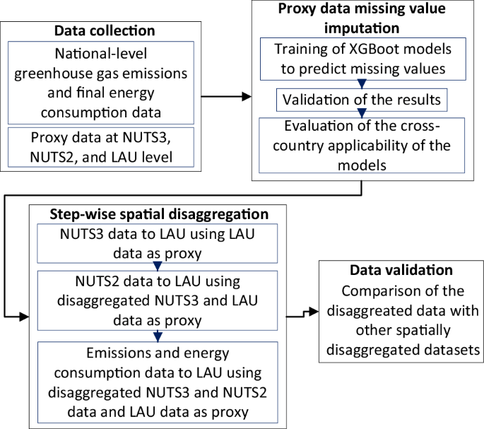
The steps involved in the spatial disaggregation of emissions and Final Energy Consumption (FEC) data from country (NUTS0) to municipal (LAU) level.
Data collection
For the disaggregation work, this study utilizes three types of data: (i) FEC data for various sub-sectors (ii) emissions data for various sub-sectors and (iii) proxy data relevant to each sub-sector, which facilitates the disaggregation of FEC and emissions data.
FEC and emissions data are collected at the national level, whereas proxy datasets are collected at various sub-national spatial resolutions. Figure 2 illustrates the Nomenclature of Territorial Units for Statistics (NUTS) spatial hierarchy in Germany and Spain. Beginning at the national level (NUTS0), the hierarchy increases in spatial resolution through successive subdivisions: NUTS1 (federal states), NUTS2 (provinces), and NUTS3 (districts). Below NUTS3, municipalities —referred to as Local Administrative Units (LAUs) —represent the most granular level of administrative geography in both countries. The size of LAUs varies significantly. In Germany, the smallest LAU is Insel Lütje Hörn, covering just 0.096 km2, while the largest is Berlin at 891.80 km2. In Spain, Emperador is the smallest LAU (0.026 km2) and Cáceres the largest (1,750.26 km2).
Fig. 2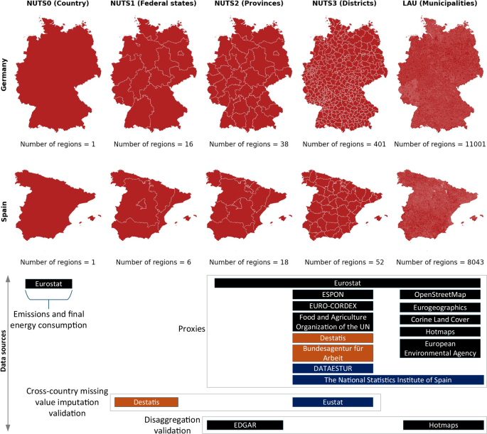
The spatial hierarchy in Germany and Spain, showing the availability of various proxy datasets from public data sources at different spatial levels. The data sources highlighted in orange and blue provide data only for Germany and Spian, respectively. Proxy data undergoes a step-wise spatial disaggregation to achieve final proxies at the LAU level. Emissions and FEC data, available at the NUTS0 level from Eurostat, is then disaggregated to LAU based on these final proxies.
The details regarding the collection of each dataset are discussed in the following sections.
Final energy consumption
The FEC data, reported at the national level, is imported from the energy balance sheet published on Eurostat15, for the year 2022. While the FEC data for both energy and non-energy use is reported on Eurostat, only the energy use FEC is considered here. The breakdown of the end-use sectors for emissions reporting on Eurostat is shown in Fig. 3.
Fig. 3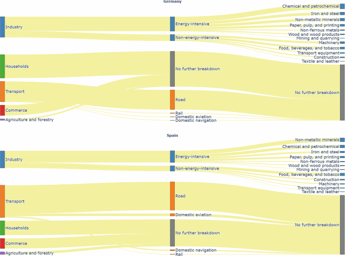
Breakdown of end-use FEC sectors as reported in Eurostat, with Germany at the top and Spain at the bottom.
The industry sector is broken down into energy-intensive and non-energy-intensive industries. Energy-intensive industries include iron and steel, chemical and petrochemical, non-ferrous metals, non-metallic minerals, mining and quarrying, paper, pulp, and printing, and wood and wood products manufacturing industries16. Non-energy-intensive industries include transport equipment, machinery, food, beverages, and tobacco, textile and leather manufacturing industries, construction, and other industries that are not specified elsewhere16. A similar categorisation is provided by Eurostat.
The transport sector is categorized into rail, road, domestic aviation, and domestic navigation. Additionally, the commerce and agriculture and forestry sectors are included, though they are not further broken down.
Greenhouse gas emissions
The GHG emissions data used in this study is sourced from Eurostat17, for the year 2022. Figure 4 illustrates how end-use sectors are categorized for emissions reporting by Eurostat. Compared to the FEC sector classification, the industry sector emissions data provided by Eurostat is less detailed. Notably, emissions from the chemical industry are not reported for Germany, and as such, these emissions are not disaggregated in this study.
Fig. 4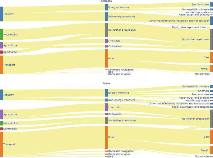
Breakdown of end-use emission sectors as reported in Eurostat, with Germany at the top and Spain at the bottom. Note: Emissions from the chemical industry are not reported for Germany on Eurostat and are therefore absent from the figure. Consequently, emissions from energy-intensive industries appear lower than those from non-energy-intensive industries.
In contrast, the transport sector is more granular in the Eurostat data compared to the FEC categorisation. Here, sub-sectors such as rail, road, domestic aviation, and domestic navigation, are further broken down into categories like light-duty trucks, heavy-duty trucks and buses, cars, and motorcycles. For the purposes of this study, emissions from light-duty trucks and heavy-duty trucks and buses are grouped under freight transport, as specific proxies for these vehicle types are not available in publicly accessible datasets.
It is important to highlight that GHG emissions in the sectors examined here primarily stem from fuel combustion. Process-related emissions in the industrial sector are excluded, with one exception: the agriculture sector, which includes non-combustion emissions. Agricultural emissions are considered under two categories-livestock and cultivation. Although Eurostat provides further disaggregation into subcategories such as enteric fermentation, manure management, agricultural soil management, and crop residue burning, only livestock and cultivation are included in this study due to the absence of matching proxies in open-source data.
Proxy data
Proxy data serves as the foundation for spatially disaggregating FEC and emissions across different end-use sectors. Unlike the FEC and emissions data, which is collected for the year 2022, proxy data spans multiple years, as certain datasets —such as land use and land cover —are not updated annually. However, all proxy datasets used represent the most recent year for which data was available at the time of collection.
The selection of proxy data was guided by the following criteria:
-
Availability in open databases: The data must be accessible through publicly available databases to enhance transparency and reproducibility.
-
Sub-national resolution: The data should be available at a sub-national scale, such as NUTS1, NUTS2, NUTS3, or LAU, to facilitate the disaggregation of emissions and FEC data reported at NUTS0.
-
Relevance to end-use sectors: The selected data must be relevant to at least one of the end-use sectors analyzed in this study. For instance, population data can be used to disaggregate household-related emissions and FEC. Heating degree days help refine the spatial distribution of FEC by accounting for higher heat demand in colder regions. In addition, industrial locations and employment data provide insights into the spatial distribution of industrial emissions and FEC. Furthermore, vehicle stock data supports the disaggregation of road transport emissions and energy consumption. Finally, land use and land cover classifications (e.g., rice fields, vineyards) assist in distributing cultivation-related FEC and emissions.
-
Data completeness: The dataset should have minimal missing values to ensure a robust analysis. Here, less than 20% missing data is preferred.
The proxies are obtained from various publicly available databases, including Eurostat, Corine Land Cover18 and OpenStreetMap. A comprehensive overview of all data sources is provided in Fig. 2. The following sub-sections provide an overview of the collected proxy data at different spatial levels, beginning with the LAU level.
Proxy data at LAU level. The datasets collected at the LAU level for Germany and Spain are summarized in Tables 1 and 2. These include general demographic and geographic statistics, such as population and area, sourced from Eurostat, which are directly available for each LAU region. However, not all relevant datasets are directly available at the LAU level. In such cases, fine-scale gridded or vector datasets are spatially overlaid with LAU geometries to derive region-specific aggregates.
Table 1 LAU-level proxy data collected from Eurostat, Hotmaps, European Environmental Agency, and The National Statistics Institute of Spain.Table 2 LAU-level proxy data collected from Corine Land Cover, Eurogeographics, and OpenStreetMap.
For example, land use and land cover information, including classes such as continuous urban fabric, is obtained from the Corine Land Cover database. This source provides raster data at a spatial resolution of 100 square meters, which allows for accurate spatial aggregation of land cover types within each LAU boundary. Similarly, air pollution data is sourced from the European Environment Agency19, available as gridded data at a resolution of 1 square kilometer.
In addition to raster sources, vector datasets are also used. The railway network data is obtained from EuroGeographics, while OpenStreetMap provides detailed information on road networks and building counts. These vector datasets are intersected with LAU geometries to extract relevant spatial indicators for each municipality.
Data on industrial sites was available in three databases: sEEnergies20, Global Steel Plant Tracker21, and Hotmaps. To determine the most suitable source, the datasets were compared for their level of detail and coverage.
-
sEEnergies provides industrial site locations along with fuel and electricity demand information for industries such as iron and steel, chemicals, non-ferrous metals, non-metallic minerals, paper and printing, and refineries.
-
Global Steel Plant Tracker focuses solely on iron and steel plant locations, annotating them with energy demand and employment data, though many sites lack complete information.
-
Hotmaps includes locations for cement and glass industries in addition to those covered by sEEnergies, with emissions data provided for each site, though data is missing for many locations.
A comparative analysis was performed to select the most comprehensive source for each sector. For the iron and steel industry, a comparison of site counts across the three datasets was conducted, as illustrated in Fig. 5. For other industries, a comparison between sEEnergies and Hotmaps was performed (see Table 3). Hotmaps reports a higher number of industrial sites across most categories, except for paper and printing industries in Germany, where sEEnergies provides higher counts. Based on this analysis, the Hotmaps database was selected as the primary source for obtaining LAU-level industry data, ensuring comprehensive coverage and consistency across sub-sectors.
Fig. 5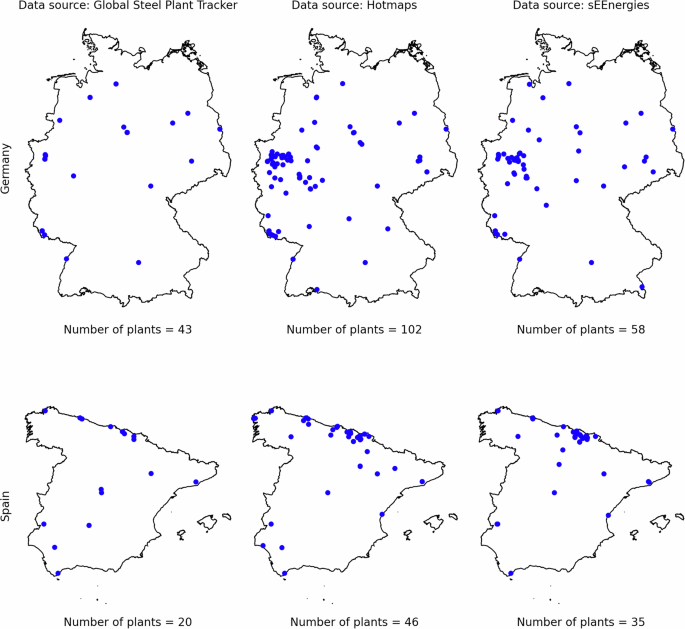
The distribution and number of iron and steel industries as reported by three open databases: Global Steel Plant Tracker, Hotmaps, and sEEnergies. The figure highlights the differences in coverage among these sources, with Hotmaps providing the most comprehensive dataset.
Table 3 Number of different industries as reported by Hotmaps and sEEnergies open databases.
Proxy data at NUTS3 level. Table 4 provides an overview of the data collected for the German and Spanish NUTS3 regions. Basic statistical information, such as employment and gross domestic product, is published by Eurostat at this spatial level. Heating and cooling degree days and livestock population datasets are available in raster format. With a resolution of approximately 10 square kilometers, these datasets align well with NUTS3 regions, enabling spatial overlap and aggregation at the NUTS3 level. Additionally, some datasets are available only in one of the two countries —for example, sectorally detailed employment data from the Federal Employment Agency22 in Germany and company counts from the National Statistics Institute of Spain23.
Table 4 NUTS3-level proxy data collected from different data sources.
Proxy data at NUTS2 level. Table 5 summarizes the data available for the German and Spanish NUTS2 regions. All the datasets collected at this level are sourced from Eurostat.
Table 5 NUTS2-level proxy data collected from Eurostat.Missing value imputation
The collected proxy datasets exhibit missing values. Imputing these values is a critical step in spatial disaggregation workflows, as complete proxy data is essential for distributing national totals. Table 6 provides an overview of the number and percentage of missing values identified in the collected proxy data. These gaps are primarily found in datasets that are available only for either Germany or Spain, often due to strict data protection regulations preventing certain regions from reporting data. Consequently, missing values must be imputed using relevant statistical indicators, such as land use and land cover data when estimating the utilized agricultural area.
Table 6 Number of missing values per variable with missing values.
To impute these missing values XGBoost model is employed. Since the spatial distribution process is relative, data quality in one region directly influences the accuracy of all others. Therefore, it is crucial to assess the model’s performance. To this end, we conduct two evaluations: (1) assessing the predictive accuracy within a country by setting aside a portion of the data for validation, and (2) evaluating the model’s predictive capacity in a country where the dataset is entirely absent. The latter is achieved by leveraging available data at intermediate spatial levels, such as states, within the country. The data sources employed in this cross-country missing value imputation evaluation are listed in Fig. 2. The training and validation of the model, as well as the evaluation of the missing value prediction across countries is explained in the following.
XGBoost model training. The datasets with missing values at the LAU level are imputed by training an XGBoost model using all other LAU-level variables as potential predictors. Before selecting the final predictors, two preprocessing steps are performed to eliminate certain variables:
-
Removal of non-informative predictors: Any predictors that have the same value across all regions are discarded because they lack predictive capability.
-
Correlation analysis: A pairwise correlation among all potential predictors is examined. If two variables exhibit an absolute correlation of 0.9 or higher, only one is retained to prevent over-representation of highly similar variables in the model.
The final dataset used as input for the XGBoost model consists of the selected predictors and the variable to be imputed, with only complete records included. Prior to training, 10% of the data is reserved for model validation, while the remaining 90% is utilized for two experimental setups. In the first setup, predictors with an absolute Pearson correlation of at least 0.1 with the variable to be imputed are included. In the second setup, the correlation threshold is increased to 0.5. Figure 6 presents the correlations between “utilized agricultural area” and the various predictors used.
Fig. 6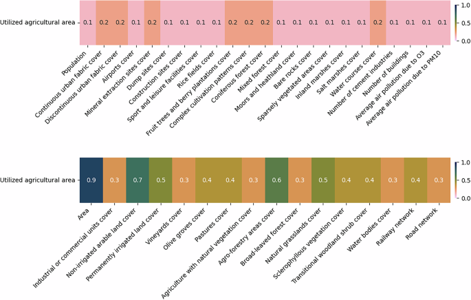
The absolute correlations between utilized agricultural area and different predictors at LAU level. The figure is divided into two sections: the top half displays the least correlated variables, while the bottom half highlights the most correlated ones. For imputing missing values in utilized agricultural area, predictors with correlations of at least 0.1 are used in one set of experiments, while those with correlations of at least 0.5 are considered in another.
In both sets of experiments, hyperparameter tuning is performed using a grid search on the XGBoost model. The hyperparameters tuned include n_estimators, learning_rate, and max_depth, with the model optimized for minimal Root Mean Squared Error (RMSE). To calculate the RMSE, 5-fold cross-validation is applied on the training data, splitting it into five folds. The RMSE is computed for each fold by training the model on four folds and validating on the remaining fold, and the average RMSE across all folds is used as the performance metric for hyperparameter optimization. The final model for data imputation is the one with hyperparameter combination that yields the lowest RMSE.
A similar approach is used in the case of variables with missing values at the NUTS3 level. Here, the potential predictors are all variables at NUTS3 level without missing values, as well as LAU variables with no missing data, aggregated to the NUTS3 level. Figures 7, 8, 9, and 10 illustrate the correlations between the NUTS3 variables with missing values and various predictors.
Fig. 7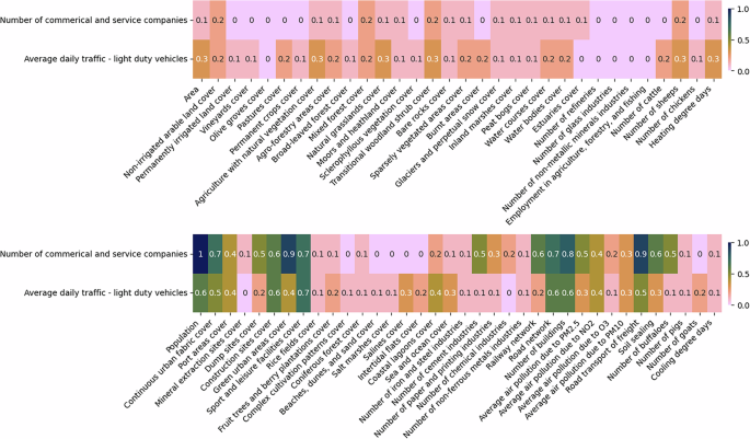
The absolute correlations between number of commercial and service companies and average daily traffic by light duty vehicles, and different predictors at NUTS3 level. The figure is divided into two sections: the top half displays the least correlated variables, while the bottom half highlights the most correlated ones. For imputing missing values, predictors with correlations of at least 0.1 are used in one set of experiments, while those with correlations of at least 0.5 are considered in another.
Fig. 8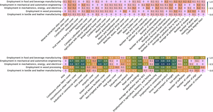
The absolute correlations between employment data and different predictors at NUTS3 level. The figure is divided into two sections: the top half displays the least correlated variables, while the bottom half highlights the most correlated ones. For imputing missing values, predictors with correlations of at least 0.1 are used in one set of experiments, while those with correlations of at least 0.5 are considered in another.
Fig. 9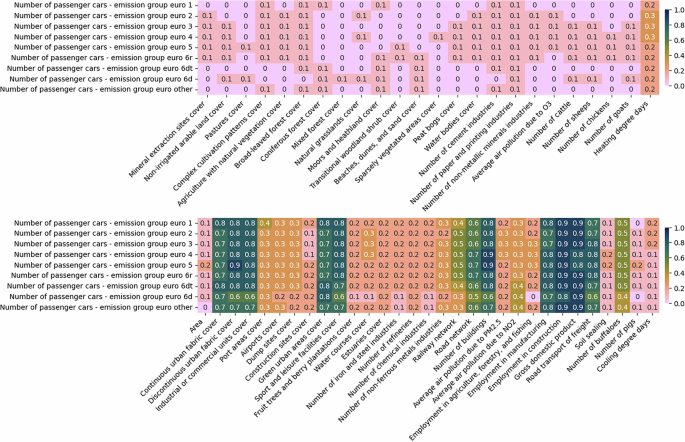
The absolute correlations between the number of passenger cars per emission group and different predictors at NUTS3 level. The figure is divided into two sections: the top half displays the least correlated variables, while the bottom half highlights the most correlated ones. For imputing missing values, predictors with correlations of at least 0.1 are used in one set of experiments, while those with correlations of at least 0.5 are considered in another.
Fig. 10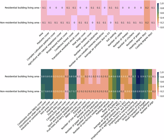
The absolute correlations between the building living area and different predictors at NUTS3 level. The figure is divided into two sections: the top half displays the least correlated variables, while the bottom half highlights the most correlated ones. For imputing missing values, predictors with correlations of at least 0.1 are used in one set of experiments, while those with correlations of at least 0.5 are considered in another.
XGBoost model validation. Table 7 presents the training and validation errors corresponding to the previously discussed correlation thresholds. While a lower RMSE indicates better model performance, its lack of fixed upper or lower bounds makes accuracy interpretation challenging. Therefore, the R-squared error is also provided, where values closer to 1 signify better performance.
Table 7 RMSE and R-squared scores on the training and validation datasets when using the XGBoost model for missing value imputation.
To ensure transparency regarding the quality of the generated values in this work, a five-level confidence schema is introduced: VERY HIGH, HIGH, MEDIUM, LOW, and VERY LOW. This qualitative labeling system facilitates easier interpretation of data quality compared to conventional statistical measures such as RMSE or R-squared values.
Confidence assignment begins at the data collection stage: all non-missing values are automatically labeled as VERY HIGH. Missing values, in contrast, are assigned one of the remaining confidence levels based on the R-squared score of the chosen imputation model. Specifically, the thresholds are defined as follows: HIGH for >0.8, MEDIUM for >0.5 and ≤0.8, LOW for >0.2 and ≤0.5, and VERY LOW for ≤0.2.
For each variable, between the two experimental settings that are considered —with correlation thresholds of ≥0.1 and ≥0.5 —the configuration yielding the higher R-squared score is selected for imputing missing values. Although the XGBoost model is trained to minimize RMSE, R-squared scores are employed for quality ratings due to their bounded range (≤1), which provides a consistent and interpretable scale across variables. The final model selected for each variable, along with its corresponding confidence level, is presented in Table 8.
Table 8 The value confidence levels assigned based on the R-squared score obtained for the better-performing model between two predictor sets: those with a correlation threshold ≥0.1 and those with a correlation threshold ≥0.5.
The trained XGBoost models effectively predict missing values for most variables (see Table 8). However, the variables “employment in the food and beverage manufacturing sector” have LOW prediction quality, and “employment in textile and leather manufacturing” is classified as VERY LOW. The poor predictions for food and beverage manufacturing can be attributed to the lack of relevant predictor data at the NUTS3 level. In addition to this limitation, the low prediction quality for textile and leather manufacturing is further exacerbated by a higher proportion of missing values, with 34 out of 401 records missing, compared to other datasets at the NUTS3 level. The variable “Average daily traffic – light duty vehicles” shows the poorest prediction results. The R-squared values are negative (see Table 7), indicating that none of the predictors contribute meaningfully to the predictions. Out of 52 records, 10 have missing values. Reserving 10% of the remaining data for validation further reduces the number of records available for training a reliable XGBoost model. Therefore, the XGBoost predictions are discarded, and missing values are imputed using the mean of the existing data. Since this approach is not robust, the imputed values are assigned a LOW prediction quality.
Evaluation of missing value prediction across countries. As previously mentioned, missing values are observed only in the country-level datasets for Germany or Spain. Consequently, the validation using the 10% of data set aside specifically assesses how well missing values can be imputed within regions of the same country. Here, the trained models are applied to predict data for regions in the other country, and the results are analyzed.
For instance, “utilized agricultural area” is available at the LAU level for Spain. A trained model, initially developed to impute missing values, is also applied to predict values for German LAU regions. These predictions are then validated against data from the Federal Statistical Office of Germany24, which provides agricultural area figures only at the NUTS1 level. To enable comparison, the predicted values are aggregated accordingly. Figure 11 demonstrates a strong alignment between the predictions and the validation data. This suggests that agricultural land use patterns in Spain and Germany are similar. The distribution of utilized agricultural area in both countries is well explained by highly correlated predictors such as total available area and non-irrigated arable land cover (Fig. 6). Given this successful validation, the XGBoost model is used to impute missing data for German LAU regions.
Fig. 11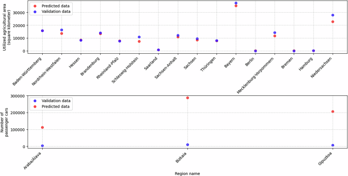
[Top] Results of training an XGBoost model to predict utilized agricultural area in Spain at the LAU level, and applying this model to estimate values for German LAU regions. The predicted data is compared with the available utilized agricultural area data at the NUTS1 level in Germany. The results indicate that the model’s predictions closely align with the actual data, with minimum and maximum deviations of 9.34 and 5106.56 square kilometers, respectively. [Bottom] Results of training an XGBoost model to predict passenger car stock in Germany at the NUTS3 level, and applying this model to estimate values for Spanish NUTS3 regions. The predicted data is compared with the available data for the 3 NUTS3 regions in the Basque Country, Spain. The results indicate that the model’s predictions deviate significantly from the actual data, with minimum and maximum deviations of 108957.0 and 276023.0 cars, respectively.
A similar validation is conducted at the NUTS3 level, where the number of passenger cars per emission group is estimated for the Spanish NUTS3 regions. The data is then aggregated into a single dataset representing the total number of passenger cars per NUTS3 region. A further aggregation to the NUTS2 level is performed, for comparison with data from Eustat25, which provides the number of cars for the three provinces of the Basque Country. Figure 11 presents this comparison, revealing significant deviations between the predictions and the validation data. A similar pattern is observed in other datasets at the German NUTS3 level. These discrepancies suggest that cross-country imputation is not universally reliable, potentially depending on the spatial level of analysis. The availability of more data at the LAU level provides greater variance, allowing for improved learning, whereas similar attempts at the NUTS3 level yield less accurate results. Additionally, sector-specific factors influence the effectiveness of imputation. For example, agricultural indicators exhibit similar spatial distributions in both countries, making cross-country imputation more feasible, whereas transport-related indicators do not follow the same pattern. Due to these inconsistencies, the predictions are discarded.
Step-wise spatial disaggregation
Figure 2 shows that only some proxy data is readily available at the LAU level, while most statistical data is typically available at NUTS3 or NUTS2 levels. Additionally, most proxy datasets do not cover the Canary Islands in Spain. Due to this limitation, these regions are excluded from the scope of this study.
In this work, we perform a step-wise spatial disaggregation. Initially, proxy data available at the NUTS3 level is disaggregated using LAU proxy data, to achieve finer resolution. Subsequently, NUTS2 proxy data is disaggregated to the LAU level using both the LAU data and the previously disaggregated NUTS3 data as proxies. Finally, the emissions and FEC data are disaggregated to the LAU level. This approach improves the accuracy of the disaggregated data by progressively refining estimates.
Among the various spatial disaggregation approaches found in the literature, proxy data-based and machine learning-based methods are the most suitable for disaggregating emissions and FEC data7. The proxy data-based approach distributes the target data based on the proportion of the chosen spatial proxy. In contrast, the machine learning-based approach trains a predictive model, such as XGBoost, to learn the relationships between all available proxy data and the target data at the source spatial level (e.g., NUTS0), and then uses this model to predict the target values in each target region.
Initially, a machine learning-based approach for disaggregation was considered. The approach was eventually discarded due to the following reasons:
-
The imputation of missing values resulted in poor predictions in certain cases. Applying an additional layer of prediction on top of this may further degrade the results.
-
In Spain, there are only 52 NUTS3 regions, which may constitute a sample size too small to generate reliable predictions at the LAU level.
-
Some variable pairs, such as population and gross domestic product, exhibited strong correlations at the NUTS3 level but weaker correlations at the LAU level. These differences in correlation raise concerns about whether the statistical relationships among variables, upon which the predictions are based, remain valid at the LAU level.
-
For most variables, no validation data is available at the LAU level, making it challenging to assess the performance of this disaggregation approach.
Therefore, in this study, a proxy data-based spatial disaggregation method is employed. Here, the quality of disaggregated data primarily depends on how effectively the chosen proxy captures the spatial distribution of the target data. The selection of a spatial proxy is inherently constrained by the availability of data at fine-scale resolution. For each target dataset, potential proxies are initially identified based on theoretical considerations. If the most suitable proxy is unavailable in open databases with sufficient non-missing values, the closest alternative is selected. For example, in disaggregating employment data for textile and leather manufacturing, the ideal proxy would be the total size of textile and leather manufacturing facilities in each LAU region. If that data is unavailable, the next best option would be the number of such facilities, followed by a broader proxy such as “industrial or commercial units cover.” Since no data on textile and leather manufacturing facilities is accessible, “industrial or commercial units cover” is ultimately chosen as the proxy.
To provide transparency regarding the reliability of the disaggregated data, each proxy is assigned a confidence level —classified as HIGH, MEDIUM, LOW, or VERY LOW —to indicate its relevance and explanatory strength with respect to the target data. The confidence level reflects the degree of alignment between the proxy and the target dataset. For instance, in the example above, the total size of textile and leather manufacturing facilities would receive a HIGH confidence rating, the number of such facilities would receive a MEDIUM rating, and “industrial or commercial units cover” would be rated as LOW.
The confidence level assigned to the final disaggregated values at the LAU level is determined by taking the minimum of the confidence level of the proxy data and that of the proxy assignment. For instance, if a proxy value in a LAU region is of MEDIUM confidence, influenced by the missing value imputation, and the proxy assignment is of LOW confidence, then the disaggregated value will be assigned a LOW confidence. The selection of proxies for the step-wise spatial disaggregation process is outlined in the following.
1. NUTS3 variables to LAU. Tables 9, 10, and 11 list the NUTS3 variables together with their potential proxies. For each variable, the most suitable proxy is first identified. If this proxy is available in any public database, it is selected and assigned a HIGH confidence level. If the most suitable proxy is unavailable, the next best alternative is considered, assigning a MEDIUM confidence level, and the process is repeated as necessary until a suitable proxy dataset is obtained for disaggregation.
Table 9 The potential proxies for disaggregating each NUTS3 variable, commonly collected for both Germany and Spain.Table 10 The potential proxies for disaggregating each NUTS3 variable, collected only for Germany.Table 11 The potential proxies for disaggregating each NUTS3 variable, collected only for Spain.
It is important to note that some proxies are added although they have different measurement units. For example “construction sites cover” and “road network” are expressed in square kilometer and kilometer. To ensure comparability, all variables are first normalized by their maximum values, preserving true zeros while scaling all other values relative to the highest observed value. This normalization allows proxies to be summed without introducing inconsistencies.
The “industrial or commercial units cover” data is sourced from the Corine Land Cover database, which includes only industrial and commercial units spanning 25 hectares or more. Due to this threshold, many regions have zero values. Since this limitation is consistent across all regions, data imputation was not feasible. Consequently, this proxy is used in conjunction with population data in this study. Furthermore, “employment in construction” uses “construction sites cover” and “road network” as proxies because construction encompasses both building and road construction.
2. NUTS2 variables to LAU. Table 12 details the proxy assignment process in the case of the NUTS2 variables “number of motorcycles”, “air transport of passengers”, and “air transport of freight”.
Table 12 The potential proxies for disaggregating each NUTS2 variable, commonly collected for both Germany and Spain.
3b. FEC (NUTS0 data) to LAU. Table 13 presents the FEC end-use sectors for which final proxies were available in both countries. Table 14 lists the FEC end-use sectors for which final proxies were available exclusively for Germany. Here, emissions from passenger car road transport are disaggregated according to the passenger car fleet categorized into different emission groups. These groups define the vehicle emission standards used in Europe26, with each group setting caps on specific air pollutants. The initial emission group, Euro 1, was introduced in July 1992. Over the years, the standards have become increasingly stringent with the introduction of new emission caps. The caps for diesel passenger cars concerning pollutants such as carbon monoxide (CO), hydrocarbons and nitrogen oxides (HC + NOX), and particulate matter (PM) are detailed in Table 15. For each emission group, the caps for these three pollutants are summed to obtain a weighting factor for the proxies. The passenger car data provides information for emission group 5 but does not differentiate between Euro 5a and 5b. In this case, the more lenient tier, Euro 5a, is considered to assign more emissions to cars in tier 5. The data also includes an emission group labeled “Other.” Due to the lack of additional information from the data source regarding this category, it is treated as the Euro 1 group. Since this data was unavailable for Spain, “average daily traffic – light duty vehicles” is used as a proxy. Similarly, Table 16 outlines the FEC end-use sectors for which final proxies were available for Spain.
Table 13 FEC end-use sectors with final proxies commonly available for both Germany and Spain.Table 14 FEC end-use sectors with final proxies available for Germany.Table 15 Emission caps for different air pollutants, per emission group.Table 16 FEC end-use sectors with final proxies available for Spain.
3a. GHG emissions (NUTS0 data) to LAU. Tables 17, 18, and 19 present the proxy assignments in the case of emissions end-use sectors. The proxies are similar to those used for FEC. The differences arise from a different breakdown of the source sub-sectors.
Table 17 GHG emissions end-use sectors with final proxies commonly available for both Germany and Spain.
In Germany, except for energy-intensive industries, all proxies correspond directly to relevant emission sources. As a result, most emissions end-use sector proxies are classified as having HIGH confidence (see Table 18). In contrast, Spain lacks detailed employment data and spatial data on residential and non-residential areas, limiting the availability of HIGH confidence proxies for several emissions end-use sectors (see Table 19).
Table 18 GHG emissions end-use sectors with final proxies available for Germany.Table 19 GHG emissions end-use sectors with final proxies available for Spain.Data validation
Finally, the spatial disaggregation results are compared with the values reported in local inventories (NetZeroCities4) and an open-source sub-national emissions dataset (EDGAR8), ensuring alignment with the sub-sectors considered in this study. The details of this validation process are presented in the technical validation section of this manuscript.