Model overview
We consider the following model to incorporate both additive and interaction effects:
$${Y}_{i}={\sum }_{j=1}^{M}{G}_{ji}{\beta }_{j}+{\sum }_{j=1}^{M}{S}_{ji}{\gamma }_{j}+{\epsilon }_{1i}{E}_{i}+{\epsilon }_{0i},$$
(1)
where \({Y}_{i}\) is the standardized phenotype adjusting the fixed effects of covariates and \({E}_{i}\) is the standardized environment variable for subject i,
$$\left[\begin{array}{c}{\beta }_{j} \\ {\gamma }_{j}\end{array}\right]\sim N([\begin{array}{c}0\\ 0\end{array}], [\begin{array}{cc}{h}_{g}^{2}/M& {\rho }_{IG}/M\\ {\rho }_{IG}/M& {h}_{I}^{2}/M\end{array}]),$$
(2)
where \({\beta }_{j}\) is the additive genetic effect size for variant j, and \({\gamma }_{j}\) is the G × E interaction effect size for variant j, \({h}_{g}^{2}\) is the narrow-sense heritability defined as the phenotypic variance explained by additive genetic effects, \({h}_{I}^{2}\) is the G × E interaction proportion, and \({\rho }_{IG}=\sqrt{{h}_{g}^{2}{h}_{I}^{2}}{r}_{IG}\) is the G × E genetic covariance between \({\beta }_{j}\) and \({\gamma }_{j}\). Here we use \({r}_{IG}\) to represent the G × E genetic correlation. For the residual term, we model:
$$[\begin{array}{c}{\epsilon }_{0} \\ {\epsilon }_{1}\end{array}]\sim N([\begin{array}{c}0\\ 0\end{array}], [\begin{array}{cc}{\sigma }_{0}^{2}& {\rho }_{01}\\ {\rho }_{01}& {\sigma }_{1}^{2}\end{array}]),$$
(3)
where \({\epsilon }_{1}\) is the residual with an interaction effect with the environmental factors and has variance \({\sigma }_{1}^{2}\), \({\epsilon }_{0}\) is the residual without an interactive effect with the environmental factors and has variance \({\sigma }_{0}^{2}\), and \({\rho }_{01}\) is the covariance between \({\epsilon }_{1}\) and \({\epsilon }_{0}\). We assume that the additive genetic effects and G × E interaction effects are polygenic. Besides, the environment variable is either non-heritable or polygenically heritable in which the additive genetic effects are uncorrelated with the G × E interaction effects on the phenotype.
Joint modeling of G × E interaction proportion and G × E genetic covariance
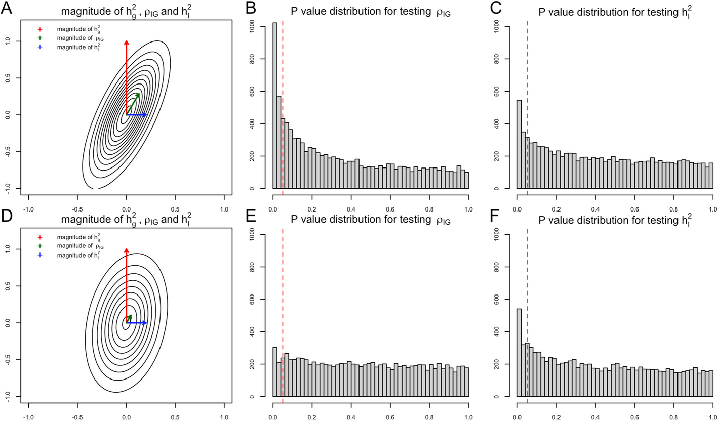
The final goal of our first task is to detect the existence of G × E interaction proportion \({h}_{I}^{2}\). Note that in a well-defined variance–covariance matrix, if one off-diagonal entry is non-zero, then it implies that its corresponding two diagonal entries are both non-zero. In the genetic random effects model, a non-zero G × E genetic covariance term \({\rho }_{IG}\) implies that both \({h}_{I}^{2}\) and \({h}_{g}^{2}\) are non-zero. Generally, the narrow-sense heritability \({h}_{g}^{2}\) has much larger magnitude than G × E interaction proportion [14], and \({\rho }_{IG}\) contains partial statistical signal from narrow-sense heritability when the G × E genetic correlation \({r}_{IG}\) is non-zero (Fig. 1). Depending on the magnitude of \({h}_{g}^{2}\), \({h}_{I}^{2}\), and \({r}_{IG}\), the statistical evidence of \({\rho }_{IG}\) is even stronger than \({h}_{I}^{2}\) in some scenarios (Fig. 1), either in simulation studies (Fig. 2) or real data analysis (Fig. 3). Several statistical methods with input of genetic summary statistics data have been developed to estimate \({h}_{I}^{2}\), \({h}_{g}^{2}\), and \({\rho }_{IG}\) [7, 11, 12, 15,16,17]. For joint modeling, we write:
$$\widehat{{\varvec{V}}}=[\begin{array}{c}\widehat{{h}_{I}^{2}} \\ \widehat{{\rho }_{IG}}\end{array}]\sim N([\begin{array}{c}{h}_{I}^{2}\\ {\rho }_{IG}\end{array}], \boldsymbol{\Sigma }),$$
(4)
where \(\boldsymbol{\Sigma }\) is the true variance–covariance matrix for the two estimates. Here we plug in the empirical variance–covariance matrix \(\widehat{\boldsymbol{\Sigma }}\) obtained via delete-block-wise jackknife. In order to indirectly test \({h}_{I}^{2}\), we propose a joint modeling test, to test the BV vector \(\left[\begin{array}{c}{h}_{I}^{2}\\ {\rho }_{IG}\end{array}\right]=\left[\begin{array}{c}0\\ 0\end{array}\right]\), which is equivalent to testing the squared Mahalanobis distance estimated by \(\widehat{{d}^{2}}={\widehat{\boldsymbol{ }{\varvec{V}}}}^{{\varvec{T}}}{\widehat{\boldsymbol{\Sigma }}}^{-1}\widehat{{\varvec{V}}}\).
Fig. 1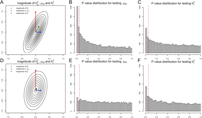
An illustration of the relationship between statistical power and magnitude of \({h}_{I}^{2}\) and \({r}_{IG}\)
Fig. 2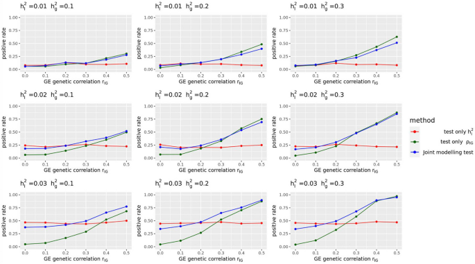
Statistical power of different GE testing methods of LDER-GE-based in simulation studies with various parameters
Fig. 3
UKBB real data analysis results for the 151 E-Y pairs
For simulation studies using real UKBB genotype data, we have a total of 54 different parameter settings, and none of the three methods dominates the other two across all parameter settings (Fig. 2). For example, when \({r}_{IG}\) is very low or equal to 0, testing only \({h}_{I}^{2}\) achieves the highest power among all three methods. On the contrary, as all parameters \({h}_{g}^{2}\), \({h}_{I}^{2}\), and \({r}_{IG}\) increase, testing only \({\rho }_{IG}\) starts to achieve higher power. And joint modeling test achieves a balance of two single-variate test methods and works the best when the true \({h}_{I}^{2}\) term is very small but \({h}_{g}^{2}\) and \({r}_{IG}\) terms are relatively large (Fig. 2). We also evaluated the type-I error rate for three tests and concluded that all three methods control the type-I error rate well (Table 1), whether they test \({h}_{I}^{2}\) directly or indirectly. Since theoretically no optimal test exists for the G × E interaction testing task across all scenarios, we applied our method to UKBB real data analysis (Methods), and the results demonstrated the efficacy of the joint modeling test (Fig. 3). Across the 151 E-Y pairs tested, there are more statistically strong (− log(p value) > 10) signals for \({\rho }_{IG}\) than \({h}_{I}^{2}\) (Fig. 3A), which can be partially attributed to the larger narrow-sense heritability of the phenotypes. Overall, testing only \({h}_{I}^{2}\) identified 35 signals, and testing only \({\rho }_{IG}\) identified 50 signals, while joint modeling test identified 63 signals, covering all signals found by the other two methods except one signal from \({\rho }_{IG}\) (Fig. 3B). A full list for all parameter estimates and p values can be found in Additional file 3: Table S1.
Table 1 Type-I error rate at 0.05 level for three LDER-GE-based methods to test \({h}_{I}^{2}\), each scenario with 500 replicationsUtilize full LD information to estimate G × E genetic covariance more accurately
We have derived the following moment condition for the product of additive genetic effect (GWAS) association vector and G × E interaction effect (GWIS) association vector (Supplementary Note 1):
$$E\left({{\varvec{Z}}}_{{\varvec{G}}}{{\varvec{Z}}}_{{\varvec{I}}}^{{\varvec{T}}}\right)=\sqrt{{N}_{G}{N}_{I}}{\rho }_{IG}{\varvec{L}}/M+2{N}_{S}\left({\rho }_{IG}+{\rho }_{01}\right){\varvec{R}}/\sqrt{{N}_{G}{N}_{I}},$$
(5)
where \({{\varvec{Z}}}_{{\varvec{G}}}\) is the Z-score vector for GWAS with sample size \({N}_{G}\), and \({{\varvec{Z}}}_{{\varvec{I}}}\) is the Z-score vector for G × E interaction effect with sample size \({N}_{I}\). Here \({N}_{S}\) is the sample overlap of two association analysis, \({\varvec{R}}\) is the LD matrix for all variants, and \({\varvec{L}}={{\varvec{R}}}^{{\varvec{T}}}{\varvec{R}}\) is the LD score matrix. We conducted eigen-decomposition on LD matrix as \({\varvec{R}}={\varvec{U}}{\varvec{D}}{{\varvec{U}}}^{T}\), where \({\varvec{D}}\) has diagonal eigenvalues and \({\varvec{U}}\) has eigenvectors and is orthogonal. We transform the original Z-score vectors as \({\widetilde{{\varvec{Z}}}}_{{\varvec{G}}}^{\boldsymbol{ }}={{\varvec{D}}}^{\left(-1/2\right)}{{\varvec{U}}}^{{\varvec{T}}}{{\varvec{Z}}}_{{\varvec{G}}}\) and \({\widetilde{{\varvec{Z}}}}_{{\varvec{I}}}^{\boldsymbol{ }}={{\varvec{D}}}^{\left(-1/2\right)}{{\varvec{U}}}^{{\varvec{T}}}{{\varvec{Z}}}_{{\varvec{I}}}\) and obtain the moment condition of the jth diagonal element of the transformed vector product:
$$E{\left({\widetilde{{\varvec{Z}}}}_{{\varvec{G}}}^{\boldsymbol{ }}{\widetilde{{\varvec{Z}}}}_{{\varvec{I}}}^{\boldsymbol{ }{\varvec{T}}}\right)}_{j,j}=\sqrt{{N}_{G}{N}_{I}}{\rho }_{IG}{D}_{j,j}/M+\frac{2{N}_{S}\left({\rho }_{IG}+{\rho }_{01}\right)}{\sqrt{{N}_{G}{N}_{I}}}.$$
(6)
The eigen-decomposition and the subsequent Z-vector transformation enable us to exploit more genetic architecture information and result in higher statistical efficiency in estimation.
Formulas (5) and (6) indicate that sample overlap between GWAS and GWIS does not affect the parameter estimates of \({{\varvec{\rho}}}_{{\varvec{I}}{\varvec{G}}}^{ }\) as \({{\varvec{N}}}_{{\varvec{S}}}\) appears only in the intercept term. This means that the GWAS and GWIS datasets can be identical, separate, or partially overlapping. In the UKBB application, the same set of individuals was used to compute both \({{\varvec{Z}}}_{{\varvec{G}}}\) and \({{\varvec{Z}}}_{{\varvec{I}}}\), consistent with this property.
Through simulations, we show that the empirical standard deviation and root mean square rate of BV-LDER-GE estimate is consistently lower than PIGEON across all simulation scenarios. The average empirical standard deviation across all simulation scenarios of BV-LDER-GE is 23.7% less than PIGEON, approximately equivalent to a sample size increase of 53% (Additional file 3: Table S2). The root mean squared error of BV-LDER-GE is also consistently lower than PIGEON across all simulation scenarios (Additional file 3: Table S2). We selected three simulation scenarios \({(h}_{I}^{2}{=0.01, h}_{g}^{2}{=0.1,r}_{IG}=0.5),{(h}_{I}^{2}{=0.02, h}_{g}^{2}{=0.2,r}_{IG}=0.5)\), and \({(h}_{I}^{2}{=0.03, h}_{g}^{2}{=0.3,r}_{IG}=0.5)\) to visualize the estimates distribution, statistical efficiency, and unbiasedness (Fig. 4). For UKBB real data, BV-LDER-GE detected G × E genetic covariance on 50 E-Y pairs while PIGEON only identified 40. For the 151 E-Y pairs, the average reported standard error of BV-LDER-GE for the 151 E-Y pairs was 30.8% lower than PIGEON (Additional file 3: Table S2), larger but consistent with simulation results.
Fig. 4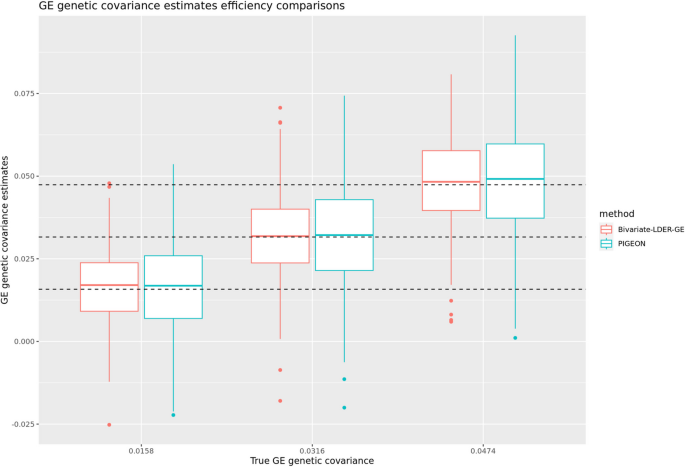
Statistical efficiency comparison of GE genetic covariance estimation for Bivariate-LDER-GE and PIGEON in simulations using real UKBB genotype panel
The authors of PIGEON [7] showed that assuming perfectly fitted PRS, the expected value of the coefficient of the PRS-by-E term in a linear regression model equals to the ratio of G × E genetic covariance and the narrow-sense heritability of the phenotype:
$$Y={\beta }_{1}PRS+{\beta }_{2}E+{\beta }_{3}PRS*E+\upepsilon ,$$
$$E\left(\widehat{{\beta }_{{3}_{\text{lm}}}}\right)=\frac{{\rho }_{GE}}{{h}_{g}^{2}}.$$
We conducted linear regression analysis on UKBB subjects using fitted PRS from external GWAS summary statistics on the 13 phenotypes and the seven environment covariates to compare the PRS-by-E regression coefficients and G × E genetic covariance estimates using BV-LDER-GE. The PRS fitting was conducted using SDPR [18]. The details for fitting PRS, linear regression, and coefficients comparison can be found in Supplementary Note 2. As shown in Fig. 5, the estimates are highly correlated (R2 = 0.808) and in all E-Y pairs where both methods are significant, the signs of PRS-by-E effects are consistent. This demonstrates the reliability of using additive genetic effect and G × E interaction summary statistics to study the PRS-by-E effect on the phenotype. Note that the estimates of the PRS-by-E regression coefficient is smaller in magnitude than estimated from BV-LDER-GE (Fig. 5, Additional file 3: Table S3) due to the attenuation bias resulted from imperfectly fitted PRS [7, 19] with measurement error. Our results indicate the potential of a more convenient and feasible alternative to evaluate the PRS-by-E effect without fitting PRS [7]. On the other hand, the p value of PRS-by-E regression test can be substantially lower than BV-LDER-GE (Additional file 3: Table S3), because BV-LDER-GE only utilizes summary-level statistics instead of individual-level genotype data. Such PRS-by-E effect direction and magnitude analysis may provide biological interpretation on how the environmental and genetic factors shape the outcome together.
Fig. 5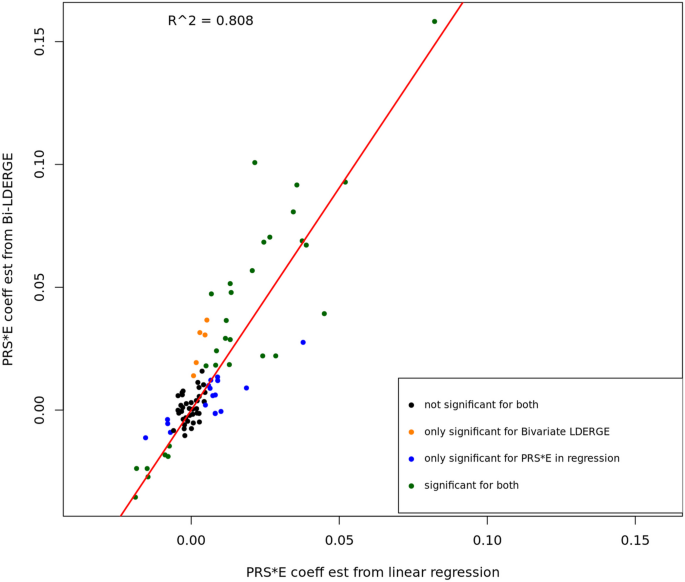
The PRS-by-E effect coefficient estimates from Bivariate-LDER-GE and linear regression
Some of our G × E interaction effect conclusions are consistent with the literature. For example, type 2 diabetes (T2D) has significant marginal PRS-by-E signals on all seven environmental covariates studies. Among them, the PRS-by-E interaction effect with sex [20, 21] and smoking [4, 22] has been reported. Meanwhile, we also report novel interaction discoveries: increased age, being a female, and having higher BMI and drinking frequency magnify the genetic effect of T2D in the European population represented by UKBB. We further ran a conditional PRS-by-E regression including all seven environmental covariates and their PRS-by-E terms in one regression model. Pm2.5 and Townsend deprivation index became nonsignificant while the other five environmental covariates remained significant with multiple testing correction (Additional file 3: Table S4). This demonstrates that multiple environmental exposures and health-related factors interact with genetic predisposition of T2D risk, which might inspire future research direction to the mechanism and intervention regarding T2D and related diseases.
Correct the confounding effects introduced by heritable environmental variable
One important assumption about the model is that the environment variable is either non-heritable or is polygenically heritable in which its additive genetic effects are uncorrelated with the G × E interaction effects on the phenotype. Many other studies consider heritable phenotypes as the interactive environmental variable [7, 23], such as BMI and alcohol intake [11, 12], and there is a need to test and correct for the potential confounding effect. PIGEON [7] developed a model and framework on this, but utilized only partial LD information through LD score regression [15]. And we improve the existing method for more accurate correction using full LD information. We write the heritable E as
$${E}_{i}={\sum }_{j=1}^{M}{G}_{ji}{\alpha }_{j}+{\epsilon }_{2},$$
(7)
the genetic random effects as
$$[ \begin{array}{c}{\beta }_{j}\\ {\gamma }_{j}\\ {\alpha }_{j}\end{array} ]{\sim }^{iid} N ( [ \begin{array}{c}0\\ 0\\ 0\end{array} ], [ \begin{array}{ccc}{h}_{g}^{2}/M& {\rho }_{IG}/M& {\rho }_{IE}/M\\ {\rho }_{IG}/M& {h}_{I}^{2}/M& {\rho }_{GE}/M\\ {\rho }_{IE}/M& {\rho }_{GE}/M& {h}_{E}^{2}/M\end{array} ] ),$$
(8)
and the moment condition for the transformed Z-score product (Supplementary Note 1),
$$E{\left({\widetilde{{\varvec{Z}}}}_{{\varvec{E}}}^{\boldsymbol{ }}{\widetilde{{\varvec{Z}}}}_{{\varvec{I}}}^{\boldsymbol{ }{\varvec{T}}}\right)}_{j,j}=\sqrt{{N}_{E}{N}_{I}}\left({\rho }_{IE}\left(1+{h}_{E}^{2}\right)\right){D}_{j,j}/M+{c}_{1},$$
(9)
$$E{\left({\widetilde{{\varvec{Z}}}}_{{\varvec{I}}}^{\boldsymbol{ }}{\widetilde{{\varvec{Z}}}}_{{\varvec{I}}}^{\boldsymbol{ }{\varvec{T}}}\right)}_{j,j}={N}_{I}\left({h}_{I}^{2}+2{{\rho }_{IE}}^{2}\right){D}_{j,j}/M+{c}_{2},$$
(10)
$$E{\left({\widetilde{{\varvec{Z}}}}_{{\varvec{G}}}^{\boldsymbol{ }}{\widetilde{{\varvec{Z}}}}_{{\varvec{I}}}^{\boldsymbol{ }{\varvec{T}}}\right)}_{j,j}=\sqrt{{N}_{G}{N}_{I}}{(\rho }_{IG}+{\rho }_{GE}{\rho }_{IE}){D}_{j,j}/M+{c}_{3},$$
(11)
where \({\widetilde{{\varvec{Z}}}}_{{\varvec{E}}}^{\boldsymbol{ }}={{\varvec{D}}}^{\left(-1/2\right)}{{\varvec{U}}}^{{\varvec{T}}}{{\varvec{Z}}}_{{\varvec{E}}}\) is the transformed Z-score vector for the GWAS on E, with sample size\({N}_{E}\), and \({c}_{s}\) are the simplified intercept terms. Identifying the slope coefficients of Eqs. (9)– (11), we iteratively estimate\({h}_{E}^{2}, {\rho }_{IE}, {h}_{I}^{2}, {\rho }_{GE}\), and \({\rho }_{IG}\) and use delete-block wise jackknife for inference. We finally use the corrected \({h}_{I}^{2}\) and \({\rho }_{IG}\) to conduct the joint modeling test on the genome-level G × E interaction proportion or estimate its magnitude directly. Our simulations showed that both BV-LDER-GE and PIGEON produce unbiased corrected estimation for G × E interaction proportion and G × E genetic covariance, but the estimation efficiency of BV-LDER-GE was 22.2% higher than PIGEON for G × E interaction proportion and 24.7% for G × E genetic covariance (Fig. 6, Additional file 3: Table S5).
Fig. 6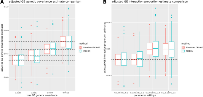
Statistical efficiency comparison of adjusted estimation of GE interaction proportion and GE genetic covariance with heritable environmental covariate confounding effects
We applied two debiased methods to the 151 E-Y pairs of UKBB dataset. Through the 151 tests, BV-LDER-GE identified 30 pairs with G × E interaction proportion bias introduced by the genetic components of the environmental variables, covering all 19 pairs of PIGEON. The confounding test is equivalent to testing term \({\rho }_{IE}\) (Eq. (10)). After adjusting for potential confounding effects, the BMI-CHO and BMI-LDL pairs failed to pass the joint modeling test of BV-LDER-GE and the rest 61 positive unadjusted BV-LDER-GE joint modeling test remained significant. The details of these 151 adjusted E-Y pairs can be found in Additional file 3: Table S6. As Fig. 7A shows, the adjusted \({h}_{I}^{2}\) estimates are always smaller than the unadjusted estimates, consistent with the theoretical derivation (Eq. (10)). And the p values will increase if the confounding effect is non-trivial (Fig. 7B). For common practice, we recommend testing the existence of term \({\rho }_{IE}\) first as some social economic status covariates may still contain genetic components [24]. If the test is significant then an adjustment of genetic confounding effect should be considered, even if a significant confounding effect may still lead to small bias (Fig. 7A).
Fig. 7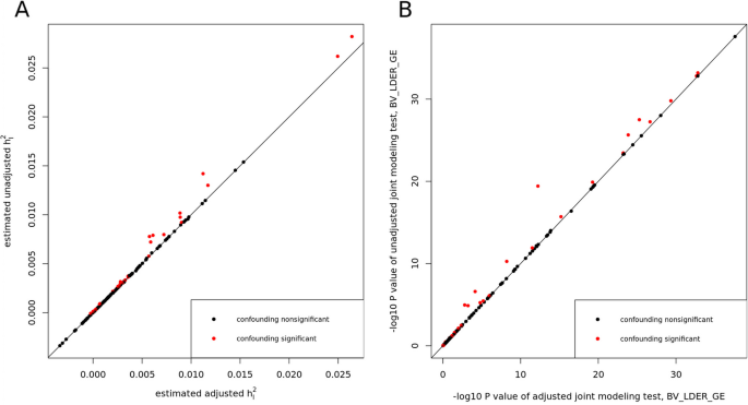
Adjusting for genetic effect of E for the 151 E-Y pairs in UKBB using BV-LDER-GE