Framework of the QRP
Before going to the QRP, we provide an overview of a brain-inspired machine-learning framework called reservoir computing36,37,38. In this paradigm, information is nonlinearly processed by networks of artificial neurons, termed the “reservoir”. A distinguishing feature is that all weight parameters within the reservoir part remain fixed, while only the output weight, which transforms the reservoir state into the final output, is trained utilizing a simple linear regression scheme. Consequently, optimization costs are markedly reduced compared to alternative schemes where the entire network weights are optimized. Importantly, due to this fixed nature, a physical system can embody the reservoir part; quantum reservoir computing (QRC) harnesses a quantum system as the reservoir (Fig. 1a)39. The quantum reservoir system evolves under the influence of the input data, and a read-out vector, constructed through repeated measurements on various degrees of freedom, undergoes linear transformation to yield the final output.
Fig. 1: Conceptualization of the QRP.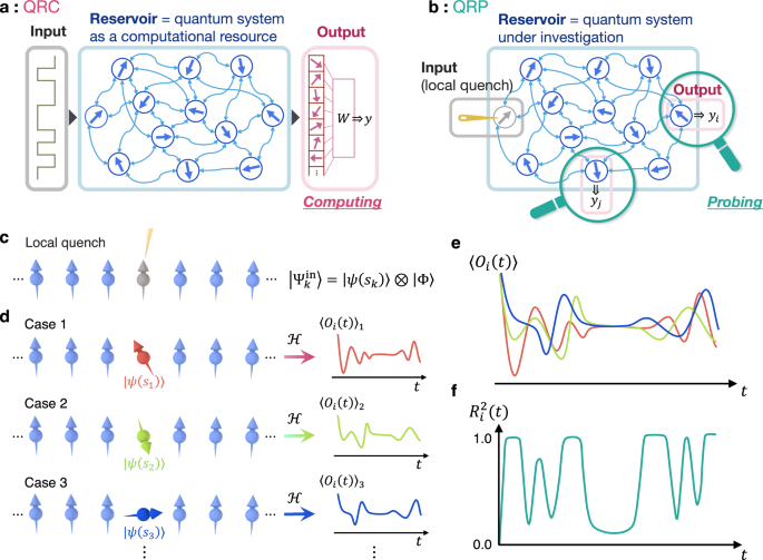
a Schematic of the QRC, which harnesses the quantum system as a computational resource. The quantum state of the reservoir reflects the provided input information, and the final output is obtained by linearly transforming a read-out vector constructed through multiple measurements on various degrees of freedom. b Schematic representation of the QRP, which investigates the quantum system from the perspective of information processing capabilities. The input is provided via the local quench, the output is calculated from local degrees of freedom, and the estimation performance of the input signifies the impact of the local quench on those degrees of freedom. c Preparation and local manipulation to construct the initial state \(\vert {\Psi }_{k}^{{{{\rm{in}}}}}\rangle\). The gray spin undergoes the local quantum quench induced by the yellow needle, while the remaining spins are initialized in the designated state \(\left\vert \Phi \right\rangle\), illustrated here as the all-up state. d Diagrammatic representation of the initial quantum state [Eq. (1)]. The central spin is locally manipulated contingent upon the input value sk for each case (three instances are depicted). This local quench induces varied dynamics in the local operator Oi(t), which is reflective of the corresponding input values. e Dynamics of 〈Oi(t)〉 summarized across three cases depicted in (d). f Schematic illustration of the determination coefficient \({R}_{i}^{2}(t)\) derived from 〈Oi(t)〉. An almost unity \({R}_{i}^{2}(t)\) signifies a precise estimation of the input value, indicating the pronounced influence of the local quench on the observed 〈Oi(t)〉 [Eq. (4)]. Conversely, \({R}_{i}^{2}(t)\) approaches zero when 〈Oi(t)〉 exhibits similar values that do not reflect each input, as exemplified by intersections of 〈Oi(t)〉.
The QRP is an inverse extension of the QRC, wherein the quantum system employed as the reservoir part is investigated by linking physical phenomena with information processing (Fig. 1b). As introduced below, the input is provided via the local quantum quench, and the output is computed from a local observable; the objective of the calculation is to estimate the original input value. Given that information is provided solely through this local quench, the estimation succeeds when the local quench exerts an influence on the observed degree of freedom. By systematically scanning local observation operators, the QRP selectively probes the impacts of the local quench on the quantum system through the input estimation performance.
The central feature underlying the QRP is the manipulation of a local degree of freedom, parametrized by a random input value sk. Our focus is on a local operator O defined at spatial position i and time t, denoted as Oi(t), with particular attention to the variations induced by the input variable sk. In the statistical analysis across various instances with different inputs subscripted by k, the expectation value \({\langle {O}_{i}(t)\rangle }_{k}\) may display diverse characteristics that closely reflect the corresponding input values. In such cases, the value of sk can be precisely deduced from \({\langle {O}_{i}(t)\rangle }_{k}\) through straightforward calculations. Hence, the successful estimation of the original input value sk provides evidence that the local manipulation exerts an influence on the operator Oi(t) at that particular spatiotemporal coordinate. In contrast, when the operator \({O}_{j}({t}^{{\prime} })\) at a different spatiotemporal point demonstrates consistent behavior across all instances, it is predominantly governed by the inherent characteristics of the quantum system independent of the local quench. Therefore, the dependency of the operator Oi(t) on the input value sk explores how the local quantum quench influences the operator while isolating it from other intrinsic phenomena. Remarkably, this linkage is highly sensitive to the Hamiltonian governing the quantum system. The operator’s dependency on the local quench operation thus serves as a witness to the properties of the quantum system, shedding light on the underlying quantum processes at play.
Here, we explain the specific procedures of the QRP on the one-dimensional (1D) quantum systems. The protocol consists of four steps: (i) the preparation of the initial state (Fig. 1c), (ii) the local quench on the central spin, parameterized by the input value sk (Fig. 1c, d), (iii) the observation of the dynamics of a local operator 〈Oi(t)〉 under the Hamiltonian \({{{\mathcal{H}}}}\) (Fig. 1d, e), and (iv) the statistical evaluation of the performance in estimating the input value sk from the observed dynamics, quantified by the determination coefficient \({R}_{i}^{2}(t)\) (Fig. 1f). We provide a comprehensive description of each step in the following.
First, the system is prepared in a designated initial state in step (i); for simplicity, a product state is assumed here (e.g., the all-up state in Fig. 1c). Subsequently, in step (ii), a specific spin undergoes a local quench manipulation based on the input value sk. The resultant state is expressed as
$$|{\Psi }_{k}^{{{{\rm{in}}}}}\big\rangle=| \psi ({s}_{k})\big\rangle \otimes \vert \Phi \rangle,$$
(1)
where \(\vert \psi ({s}_{k})\rangle\) represents the state of the locally manipulated spin, while \(\vert \Phi \rangle\) denotes the prepared initial state for the remaining subsystem (Fig. 1d). The input value sk is randomly sampled from a uniform distribution, specifically sk ∈ [0, 1]. For instance, we consider the initial state as
$$\vert \psi ({s}_{k})\rangle=\sqrt{1-{s}_{k}}\vert+\rangle+\sqrt{{s}_{k}}\vert -\rangle,$$
(2)
where \(\vert \pm \rangle=\left(\vert \uparrow \rangle \pm \vert \downarrow \rangle \right)/\sqrt{2}\). This state can be prepared by applying a single-gate pulse or a local magnetic field \({{{\bf{h}}}}\propto (2{s}_{k}-1,0,-2\sqrt{{s}_{k}(1-{s}_{k})})\).
We then let the system evolve under the Hamiltonian \({{{\mathcal{H}}}}\) in step (iii), resulting in the state \(\vert {\Psi }_{k}(t)\rangle={e}^{-i{{{\mathcal{H}}}}t}\vert {\Psi }_{k}^{{{{\rm{in}}}}}\rangle\) (see Methods section). The expectation value of a local operator Oi(t) is calculated as \({\langle {O}_{i}(t)\rangle }_{k}=\langle {\Psi }_{k}(t)| {O}_{i}| {\Psi }_{k}(t)\rangle\); we omit the subscript k unless necessary. By iterating this procedure across various instances with different sk, we generate multiple time series of the dynamics, as illustrated in Fig. 1e.
Finally, in step (iv), we assess the influence of the local quantum quench on the local operator. As a criterion, we employ precision in estimating the input value sk through the linear transformation of \({\langle {O}_{i}(t)\rangle }_{k}\), following the standard methodology used in reservoir computing paradigm35,36,37,38,39. For a given instance k, the output of this linear transformation is derived as
$${y}_{i,k}(t)={w}_{i,O}(t){\langle {O}_{i}(t)\rangle }_{k}+{w}_{i,c}(t),$$
(3)
where wi,O(t) and wi,c(t) represent the k-independent coefficients. These weights are finely tuned for training instances so that the output yi,k(t) approximates the original input value sk as closely as possible over all k, based on the least squares method. Subsequently, in the testing phase, the estimation performance for unknown instances is quantified by the determination coefficient
$${R}_{i}^{2}(t)=\frac{{{{{\rm{cov}}}}}^{2}(\{{y}_{i,k}(t)\},\{{s}_{k}\})}{{\sigma }^{2}(\{{y}_{i,k}(t)\}){\sigma }^{2}(\{{s}_{k}\})},$$
(4)
where cov and σ2 represent covariance and variance, respectively; see Methods section for more details. The value of \({R}_{i}^{2}(t)\) ranges between 0 and 1, with an approach towards 1 indicating that the outputs {yi,k(t)} closely reproduce the inputs {sk} for all testing instances.
Figure 1e, f visually elucidate the relationship between the dynamics of \({\langle {O}_{i}(t)\rangle }_{k}\) and the corresponding \({R}_{i}^{2}(t)\). A high \({R}_{i}^{2}(t)\) value suggests that \({\langle {O}_{i}(t)\rangle }_{k}\) varies systematically in response to the input value sk. In contrast, \({R}_{i}^{2}(t)\) close to 0 indicates that \({\langle {O}_{i}(t)\rangle }_{k}\) is largely independent of sk, such as at the crossing points resulting from intrinsic oscillations in the quantum system. Therefore, \({R}_{i}^{2}(t)\) serves as an indicator of the extent to which Oi(t) is influenced by the local quench operation. Under different parameters of the Hamiltonian \({{{\mathcal{H}}}}\), the local quench operation exerts varying influences on the resultant dynamics, hence the behavior of \({R}_{i}^{2}(t)\) is instrumental in examining the unique properties of each quantum phase. It is worth noting that, although the input in Eq. (2) includes a nonlinear contribution from sk, our analysis concentrates on the spatiotemporal dynamics of the linear component in accordance with the QRC framework. Any additional complexity beyond linear regression could impede interpretability, as the output is influenced by the extraneous characteristics of the transformation itself.
Transverse-field Ising model
Let us first apply our QRP protocol to the paradigmatic 1D Ising model with a transverse magnetic field under the open boundary condition. The Hamiltonian is given by
$${{{\mathcal{H}}}}=-J{\sum}_{i}{\sigma }_{i}^{z}{\sigma }_{i+1}^{z}+g{\sum}_{i}{\sigma }_{i}^{x},$$
(5)
where \({\sigma }_{i}^{x}\) and \({\sigma }_{i}^{z}\) are the x and z Pauli matrices at site i, respectively. g signifies the magnitude of the transverse magnetic field, and J > 0 denotes the strength of the nearest-neighbor ferromagnetic interaction; we set J = 1 as our energy scale. This model manifests a quantum phase transition at the quantum critical point gc = 1 in the thermodynamic limit, which separates a ferromagnetically ordered phase for g g > 11,40. Notably, the model is solvable through the Jordan-Wigner transformation and the subsequent Bogoliubov transformation, where the spin system is mapped to the free quasiparticle picture1.
In step (i), the system is initialized in the all-up state, and after the local quantum quench at the central spin in step (ii), the resultant state \(\vert {\Psi }_{k}^{{{{\rm{in}}}}}\rangle\) in Eq. (1) is explicitly expressed as
$$\big| {\Psi }_{k}^{{{{\rm{in}}}}}\big\rangle=\vert \uparrow \uparrow \uparrow \ldots \,\rangle \otimes \vert \psi ({s}_{k})\rangle \otimes \vert \uparrow \uparrow \uparrow \ldots \,\rangle,$$
(6)
using \(\vert \psi ({s}_{k})\rangle\) defined in Eq. (2). In step (iii), we monitor the dynamics of the local spin \(\langle {\sigma }_{i}^{x}(t)\rangle\) at each site i under the Hamiltonian \({{{\mathcal{H}}}}={{{\mathcal{H}}}}(g)\). Repeating the procedure for many instances with varying sk, the estimation performance \({R}_{i}^{2}(t)\) in Eq. (4) is methodically evaluated in step (iv).
Figure 2 encapsulates the results of the QRP under various magnetic fields g. In Fig. 2a, we show the spatiotemporal representation of the estimation performance \({R}_{i}^{2}(t)\), which reveals a discernible light-cone structure emanating from the quenched central site. The broad distribution of nonzero \({R}_{i}^{2}(t)\) suggests that the local spin operator \(\langle {\sigma }_{i}^{x}(t)\rangle\) across diverse spatial locations and temporal moments adequately reflects the impact of the local quantum quench. In the quantum disordered phase, where the ground state exhibits spins aligned along the x direction, the effects of the local quench along the x axis in spin space propagate akin to a spin wave, characterized by pronounced wavefronts of \({R}_{i}^{2}(t)\). In contrast, in the ferromagnetically ordered phase, the local quenching effects are preserved predominantly within the quasiparticles, manifesting as alterations in phase and amplitude. This influence is evidenced by the ripple-like patterns of the nonzero \({R}_{i}^{2}(t)\). An exception occurs near the quantum critical point at gc = 1, characterized by maximized fluctuations that lead to an effective breakdown of the quasiparticle picture. Here, the effects of the local quench are passed on to the intrinsic fluctuations of the system, though such influences rapidly diminish as indicated by the noticeably small \({R}_{i}^{2}(t)\) after the passage of the wavefront. This observation highlights an anomalous suppression of the local quenching effects at the quantum critical point, which is distinct from those in other non-critical phases.
Fig. 2: Identifying the quantum phase transition in the transverse-field Ising model via the QRP.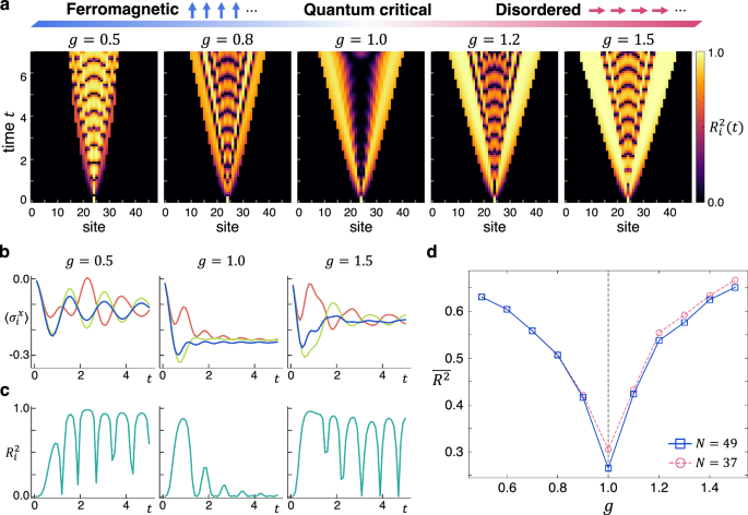
a Spatiotemporal representation of the performance for the estimation of the input value. The color represents the value of \({R}_{i}^{2}(t)\) derived from \(\langle {\sigma }_{i}^{x}(t)\rangle\). The upper band represents the schematic phase diagram regarding \({{{\mathcal{H}}}}(g)\), where the quantum critical point separating the ferromagnetically ordered phase and the quantum disordered phase exists at gc = 1. The system size is N = 49, and the time evolution is calculated using a bond dimension χ = 256; the result is quantitatively the same for χ = 128. b The early-time spin dynamics at the nearest neighbor site from the central one under three different input values. c The estimation performance \({R}_{i}^{2}(t)\) utilizing \(\langle {\sigma }_{i}^{x}(t)\rangle\) at the same site as (b). d The average \(\overline{{R}^{2}}\) over spatiotemporal indices (i, t) ∈ Λ × {0 t ≤ 7}, with Λ encompassing the central nine sites. The blue and pink lines represent the results for system sizes N = 49 and N = 37, respectively, exhibiting analogous behavior. The quantum critical point is denoted by the gray dashed line.
In Fig. 2b, the early-time dynamics of \(\langle {\sigma }_{i}^{x}(t)\rangle\) at the nearest-neighbor spin from the central one is depicted for three distinct input values sk at different magnetic fields g. At g = 0.5 and 1.5, periodic spin oscillations are induced, with their phase and amplitude dependent on the input sk. In contrast, at g = 1.0, the dynamics of \(\langle {\sigma }_{i}^{x}(t)\rangle\) exhibits significant variation when the wavefronts pass at approximately t ≃ 1, thereafter stabilizing into a featureless pattern with diminished influence from the quench operation. Figure 2c displays the corresponding estimation performance at the same site (a vertical cross-section of the color map in Fig. 2a). Over broad temporal spans at g = 0.5 and 1.5, \({R}_{i}^{2}(t)\) becomes close to 1, which statistically underscores the input dependency of the phase and amplitude of the spin oscillations. In contrast, their frequency is governed not by the local quench on the initial state, but rather by the intrinsic characteristics of the quasiparticles themselves. This is evidenced by \({R}_{i}^{2}(t)\) periodically approaching zero (Fig. 2c) at points where oscillations of \(\langle {\sigma }_{i}^{x}(t)\rangle\) intersect for different inputs (Fig. 2b). Notably, at g = 1.0, while \({R}_{i}^{2}(t)\) nears 1 around t ≃ 1 where the wavefronts induce variations in the spin dynamics, \({R}_{i}^{2}(t)\simeq 0\) in other temporal regions signifies the reduced influence of the local quench due to the intrinsic fluctuations enhanced near the quantum critical point.
As described above, the effects of the local quantum quench on the resultant dynamics of local operators manifest qualitatively different characteristics across various phases (Fig. 2a). The distribution of \({R}_{i}^{2}(t)\) thus serves as a marker for identifying the quantum phase transition. To enhance the clarity of the results, in Fig. 2d, we display the mean value of \({R}_{i}^{2}(t)\) over a specific subset of spatiotemporal indices {(i, t)}, denoted as \(\overline{{R}^{2}}\). This analysis focuses on (i, t) within the central nine sites during the time interval 0 t ≤ 7; selecting different subsets does not qualitatively alter the results (see the Supplementary Information). We note that \(\overline{{R}^{2}}\) represents a simple average of local quantities, and therefore, does not include nonlocal quantum effects. As g approaches gc = 1 from the ferromagnetically ordered state, the fluctuations progressively intensify and interfere with the estimation of the original input, resulting in a decrease in \(\overline{{R}^{2}}\). At the quantum critical point, \(\overline{{R}^{2}}\) reaches its minimum, which corresponds to the emergence of a dark region between the wavefronts observed in Fig. 2a for g = 1.0. Upon further augmentation of g into the quantum disordered phase, the fluctuations weaken again and the effects of the quench operation become dominant, leading to an increase in \(\overline{{R}^{2}}\). The pronounced dip in Fig. 2d is, therefore, a definitive indicator of the quantum phase transition occurring at g = gc. Consequently, by focusing on the effects of the local quantum quench, our QRP successfully detects the quantum phase transition only by measurements of single-site spin dynamics.
Anisotropic next-nearest-neighbor Ising model
To illustrate the applicability of our QRP framework to nonintegrable systems, we extend the model to the anisotropic next-nearest-neighbor Ising (ANNNI) chain41,42,43,44. The Hamiltonian is given by
$${{{\mathcal{H}}}}=-J{\sum}_{i}{\sigma }_{i}^{z}{\sigma }_{i+1}^{z}-\kappa {\sum}_{i}{\sigma }_{i}^{z}{\sigma }_{i+2}^{z}+g{\sum}_{i}{\sigma }_{i}^{x},$$
(7)
where J and κ represent the strengths of the nearest-neighbor and the next-nearest-neighbor interactions, respectively; we take J = 1. The latter term makes the system nonintegrable by introducing the four-body interactions for the quasiparticles derived by the Jordan-Wigner transformation. This model hosts a rich phase diagram in the κ-g plane45. Our investigation focuses on the case of κ = 0.5, where the quantum phase transition occurs at g = gc with the Ising universality, separating ferromagnetically ordered (g gc) and quantum disordered (g > gc) phases. In our finite-size system with open boundary conditions, we determined gc ≃ 1.7 utilizing the density matrix renormalization group (DMRG) method. The initial state is prepared in the same manner as Eq. (6).
Figure 3a displays the spatiotemporal representation of \({R}_{i}^{2}(t)\) obtained from \(\langle {\sigma }_{i}^{x}(t)\rangle\), revealing a scenario similar to the transverse-field Ising model. For the majority of sites and times, the local spin \(\langle {\sigma }_{i}^{x}(t)\rangle\) mirrors the input value sk employed in the local quantum quench, as evidenced by the nonzero values of \({R}_{i}^{2}(t)\). Above the critical field at gc ≃ 1.7, particularly for g = 2.6 in the right panel, the effects of the local manipulation propagate primarily through the excitation wavefronts, while the local spin oscillations exhibit weaker dependence on the local quench with small \({R}_{i}^{2}(t)\). Conversely, below the critical point, the opposite behavior is noted in the left panel for g = 1.0. Furthermore, in the vicinity of the quantum critical point, the influence of the local quench manifests itself predominantly along the wavefronts, while in the other regions it is suppressed by the enhanced quantum fluctuations, as demonstrated by the emergence of a discernible dark zone between the wavefronts. These fundamental dependencies of the local spin operators on the local quench retain a similarity to those observed in the integrable model presented in Fig. 2a.
Fig. 3: Detection of the quantum phase transition in the ANNNI model using the QRP.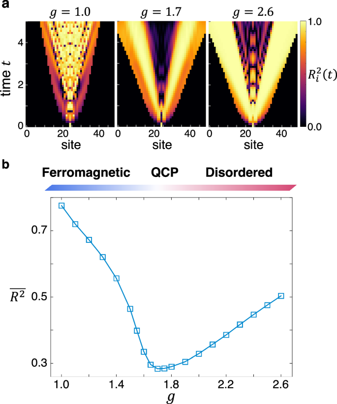
a Spatiotemporal representation of the estimation performance when employing \(\langle {\sigma }_{i}^{x}(t)\rangle\) in the nonintegrable ANNNI chain characterized by the interaction parameter κ = 0.5. The system size is N = 49, and the time evolution is calculated with a bond dimension of χ = 256. b The average \(\overline{{R}^{2}}\) over a subset (i, t) ∈ Λ × {0 t ≤ 5}, where Λ contains the central seven sites. The upper band represents the schematic phase diagram, where the ferromagnetically ordered and quantum disordered phases are separated by the quantum critical point at approximately gc ≃ 1.7.
In Fig. 3b, we present the mean value \(\overline{{R}^{2}}\), calculated over the indices (i, t) corresponding to the central seven sites within the time frame 0 t ≤ 5 (see the Supplementary Information for other subsets). Analogous to the observation in Fig. 2d, \(\overline{{R}^{2}}\) demonstrates a pronounced decrease around the quantum critical point at gc ≃ 1.7, precisely locating the boundary between the different spatiotemporal distribution patterns of \({R}_{i}^{2}(t)\) in the ferromagnetically ordered phase and the quantum disordered phase. This observation confirms that, even in nonintegrable quantum systems, \({R}_{i}^{2}(t)\) functions as an effective marker for detecting quantum phase transitions.
Cluster model
The preceding sections have demonstrated the effectiveness of our QRP in identifying quantum phase transitions, particularly between conventional phases where the internal physics is well-characterized and understood within the Landau-Ginzburg-Wilson theory. Building on this foundation, we now aim to broaden our exploration to more complex quantum phenomena. In particular, we apply the QRP framework to the detection of topological quantum phase transitions, which lack local order parameters that can distinguish adjacent phases. This raises the question of whether the QRP framework, which solely utilizes a single-site spin operator, can still be effective in identifying these transitions beyond the Landau-Ginzburg-Wilson paradigm.
Here, we study the cluster model with open boundaries46,47,48, which is defined by
$${{{\mathcal{H}}}}=-{\sum}_{i}{J}_{zz}{\sigma }_{i}^{z}{\sigma }_{i+1}^{z}+{\sum}_{i}{J}_{zxz}{\sigma }_{i}^{z}{\sigma }_{i+1}^{x}{\sigma }_{i+2}^{z},$$
(8)
where Jzz and Jzxz denote the Ising and cluster interaction strengths, respectively; we set Jzz = 1. This model is renowned for hosting a symmetry-protected topological (SPT) phase, known as the cluster state, which emerges for Jzz Jzxz. The SPT phase is distinguished by its protection under a \({{\mathbb{Z}}}_{2}\times {{\mathbb{Z}}}_{2}^{T}\) symmetry, and is characterized by nonlocal string order parameters49,50,51,52,53. As the strength of the cluster interaction diminishes, the quantum phase transition occurs from the SPT phase to the topologically trivial, ferromagnetically ordered phase at the quantum critical point Jzxz = 1. We aim to detect this transition through the dynamical signature in the QRP, by preparing the initial state in Eq. (6) and monitoring the dynamics of the local spin \({\sigma }_{i}^{x}(t)\).
In Fig. 4a, we present the estimation performance \({R}_{i}^{2}(t)\) under the Hamiltonian \({{{\mathcal{H}}}}\) for three different strengths of the cluster interaction: Jzxz = 0.6 in the ferromagnetically ordered phase, Jzxz = 1.4 in the SPT phase, and Jzxz = 1.0 at the quantum critical point. Consistent with the previous topologically trivial models, the spread of nonzero \({R}_{i}^{2}(t)\) values indicates that the operator \({\sigma }_{i}^{x}(t)\) is reflective of the local quantum quench at various spatiotemporal points. Importantly, at the quantum critical point, a notable trend is observed wherein \({R}_{i}^{2}(t)\) is suppressed following the passage of the wavefronts. This precisely mirrors the trend observed at the quantum critical point in conventional quantum phase transitions (Figs. 2d and 3b).
Fig. 4: Probing the quantum phase transition between the ferromagnetically ordered and SPT phases in the cluster model using the QRP.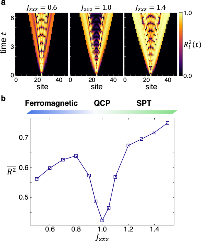
a Spatiotemporal representation of the estimation performance \({R}_{i}^{2}(t)\) employing \(\langle {\sigma }_{i}^{x}(t)\rangle\) for a system with N = 49 sites. The time evolution is calculated with a bond dimension of χ = 256. b The average \(\overline{{R}^{2}}\) over a subset (i, t) ∈ Λ × {0 t ≤ 6.5}, where Λ represents the central eleven spins. The upper bar illustrates the phase diagram.
Figure 4b presents the mean value \(\overline{{R}^{2}}\), which effectively distinguishes these three distinct distributions of \({R}_{i}^{2}(t)\). \(\overline{{R}^{2}}\) is computed as the average of \({R}_{i}^{2}(t)\) for the central eleven spins within the time interval 0 t ≤ 6.5. A key observation in Fig. 4b is the pronounced dip at \({{J}_{zxz}}=1.0\), signifying the suppression of the impact of local quantum quench. This dip thus marks the quantum critical point characterized by enhanced quantum fluctuations, clearly delineating the boundary between the SPT phase and the trivial ordered phase. Therefore, despite the absence of local order parameters in the topological phase, our QRP, based on the local quench and local observables, demonstrates itself as a potent instrument for detecting the topological quantum phase transition.
Cluster model in a magnetic field
Finally, we extend the cluster model in Eq. (8) by introducing a transverse magnetic field:
$${{{\mathcal{H}}}}=-{J}_{zz}{\sum}_{i}{\sigma }_{i}^{z}{\sigma }_{i+1}^{z}-{h}_{x}{\sum}_{i}{\sigma }_{i}^{x}+{J}_{zxz}{\sum}_{i}{\sigma }_{i}^{z}{\sigma }_{i+1}^{x}{\sigma }_{i+2}^{z}.$$
(9)
The interplay among these three terms gives rise to a complex phase diagram54,55,56,57: the SPT phase is stabilized when the cluster interaction term dominates with a large Jzxz, while topologically trivial phases emerge in the ferromagnetically ordered state under strong Ising interaction or in the disordered state under a strong magnetic field. Here, we fix Jzz = 0.1 and vary Jzxz = (1 − Jzz)α and hx = (1 − Jzz)(1 − α), with a tuning parameter α adjusting the balance between the cluster and magnetic field terms. At the critical value αc = 0.5, the topological quantum phase transition occurs, delineating the SPT phase (α > αc) from the disordered phase (α αc)57. Importantly, these phases are devoid of local orderings on both sides of the quantum critical point, unlike the transition examined in Fig. 4, which exhibits the local ferromagnetic order on one side. We initialize the system as
$$\big| {\Psi }_{k}^{{{{\rm{in}}}}}\big\rangle=\big| {+}_{y}{+}_{y}\cdots \,\big\rangle \otimes \big| {\psi }^{{\prime} }({s}_{k})\big\rangle \otimes \big| {+}_{y}{+}_{y}\cdots \,\big\rangle,$$
(10)
where \(\vert {\psi }^{{\prime} }({s}_{k})\rangle=\sqrt{1-{s}_{k}}\vert {+}_{y}\rangle+\sqrt{{s}_{k}}\vert {-}_{y}\rangle\) and \(\vert {\pm }_{y}\rangle=\left(\vert \uparrow \rangle \pm i\vert \downarrow \rangle \right)/\sqrt{2}\). \({R}_{i}^{2}(t)\) is subsequently evaluated from the dynamics of \({\sigma }_{i}^{x}\). These are chosen to clearly demonstrate the QRP by leveraging the flexibility of both the input and output.
Figure 5a illustrates the estimation performance \({R}_{i}^{2}(t)\) under the Hamiltonian \({{{\mathcal{H}}}}\) for three different values of α. In all scenarios, \({R}_{i}^{2}(t)\) acquires nonzero values propagating from the central site throughout the system, where the distinctions between the phases become evident. Notably, at the quantum critical point (α = αc), \({R}_{i}^{2}(t)\) is markedly suppressed, displaying a discernibly dark spatiotemporal region in Fig. 5a. This behavior contrasts with the SPT phase at α = 0.7 and the trivial disordered phase at α = 0.3, both of which exhibits more complicated pattern with widely spread nonzero \({R}_{i}^{2}(t)\). To quantitatively assess these differences, we illustrate the α dependence of \(\overline{{R}^{2}}\) in Fig. 5b, which is defined by averaging \({R}_{i}^{2}(t)\) over the central 13 sites within the time frame 0 t ≤ 7. Consistent with the previous models, \(\overline{{R}^{2}}\) exhibits a pronounced dip at the quantum critical point, which precisely delineates the boundary between the trivial and topological phases. Indeed, the quantum fluctuations are consistently amplified near the critical point, irrespective of the system’s topological nature or the existence of local orderings. Therefore, even purely topological quantum phase transitions can be detected via the QRP, using these fluctuations in the post-local quench dynamics as witnesses.
Fig. 5: Detection of the disordered-to-SPT quantum phase transition in the cluster model under a magnetic field via the QRP.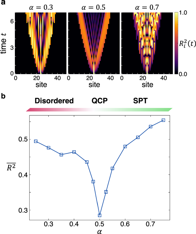
a Color map of the estimation performance \({R}_{i}^{2}(t)\) for \(\langle {\sigma }_{i}^{x}(t)\rangle\) in the cluster model under a magnetic field with Jzxz = (1 − Jzz)α, hx = (1 − Jzz)(1 − α), and Jzz = 0.1, The system size is N = 49, and the time evolution is calculated with a bond dimension of χ = 256. b The average \(\overline{{R}^{2}}\) over a subset (i, t) ∈ Λ × {0 t ≤ 7}, where Λ contains the central 13 sites. The upper band represents the phase diagram, where the topological and disordered phases are separated by the quantum critical point at α = 0.5.