Magnetic hysteresis switching in trilayer CrSBr devices
Figure 1a shows the structure of a 3L CrSBr back-gate device. The 3L CrSBr is covered by a monolayer graphene, which also contacts the two gold (Au) electrodes positioned on either side of the CrSBr. These electrodes allow to monitor the charge neutral point in graphene. A thin flake of hexagonal boron nitride (hBN) is encapsulated on top of the graphene/CrSBr heterostructure as a protective capping layer. Since the exchange interaction in CrSBr is highly sensitive to strain21, the 3L CrSBr is exfoliated directly onto the substrate without any pickup process during dry transfer. This approach minimizes strain-induced inhomogeneity in the CrSBr. The entire exfoliation and encapsulation are performed in a glove box under a nitrogen atmosphere to prevent potential contamination of the sample.
Fig. 1: Magneto-PL measurements of 3L CrSBr device.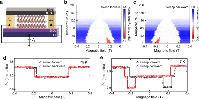
a Schematic of 3L CrSBr device. The monolayer graphene (1L Gr) is contacted with two Au electrodes for monitoring its charge neutral point. The back gate voltage (Vg) is applied to the silicon substrate. Temperature dependent PL intensity loops from 200 K to 7 K, with the magnetic field sweeping forward (b) and backward (c) along the easy axis. The PL intensity is normalized as detailed in Supplementary Note 1. PL hysteresis loops at 75 K (d) and 7 K (e).
The coupling of magnetic structures and exciton emission in CrSBr allows for the investigation of magnetic transitions via PL characterization10,18,22. We first employ magneto-PL measurements at various temperatures. Figure 1b, c present the PL intensity loops as the magnetic field sweeps from −0.4 T to 0.4 T (forward) and vice versa (backward) along the easy axis (b-axis), across a temperature range from 200 K to 7 K. The PL intensity is integrated from the exciton emission within the energy range from 1.24 eV to 1.38 eV. To highlight the intensity switching, the temperature-dependent PL loops are normalized by using the intensity difference between 0 T and 0.4 T at 7 K (see Supplementary Fig. 1 and Supplementary Note 1). Above the Néel temperature (TN) at ~135 K9,10,19,23,24, the 3L CrSBr exhibits a paramagnetic state, with no PL intensity switching observed during magnetic field sweeps. Between 135 K and 40 K, the PL loops reveal two distinct intensity levels, as demonstrated by a representative loop at 75 K in Fig. 1d. These levels correspond to different magnetic states, with layered AFM states appearing at low magnetic fields and FM states emerging at high fields10,20.
Notably, a new lower-intensity level emerges below 40 K, as illustrated by the loop at 7 K (Fig. 1e). To further differentiate the three PL intensity levels in 3L CrSBr device, we obtain the excitonic PL spectra. As depicted in Fig. 2a, the spectra at ±0.4 T exhibit a single excitonic peak at 1.328 eV. At 0 T, the PL spectra display two separate excitonic peaks at 1.338 eV and 1.363 eV. These observations are consistent with previous studies10,22, where the spectra at ±0.4 T correspond to FM states and those at 0 T correspond to AFM states. By contrast, the spectra at ±0.2 T both show a single peak at 1.338 eV, which differ from those of the FM and AFM states. The corresponding PL images confirm the uniformity and high quality of our samples (Fig. 2a, insets). These observations suggest that the new PL level corresponds to an unidentified type of magnetic states. The PL results are reproduced in an additional 3L CrSBr device S2, as shown in Supplementary Fig. 2.
Fig. 2: Magnetic SHG of the 3L CrSBr device.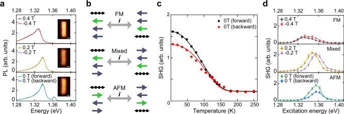
a PL spectra at ±0.4 T (top), ±0.2 T (middle) and ±0 T (bottom), respectively. The insets are the corresponding PL microscopic images. Scale bar, 2 μm. b Symmetry analysis of the lattice structure and the FM (top), Mixed (middle), and AFM (bottom) structures of 3L CrSBr. The spatial-inversion operation is denoted by the symbol i. The CrSBr layer with charge transfer from the contacted graphene is marked by the green arrows. The charge transfer breaks the inversion symmetry of the lattice and FM, Mixed, and AFM states under the spatial-inversion operation i. c Temperature dependence of SHG intensity for the two AFM states. The red and black solid curves are shown as a guide for the eye. d SHG excitation spectra at ±0.4 T (top), ±0.2 T (middle), and ±0 T (bottom), respectively.
To better understand the emergent states, we categorize all possible magnetic structures, as summarized in Supplementary Table 1. The magnetic states can be classified into three types based on interfacial magnetization: FM states (M = ±3) with two FM vdW interfaces, AFM states (M = ±1) with two AFM interfaces, and Mixed states (M = ±1) with one FM and one AFM interfaces. Here, M denotes the total magnetization of the three CrSBr layers, where the magnetization in each monolayer is represented by left and right arrows, corresponding to M = −1 and 1, respectively. Within each category, the magnetic configurations share equivalent interlayer magnetic arrangements, resulting in identical excitonic PL emission. Thus, the three types of PL spectra can be attributed to the FM, Mixed and AFM states, with the states at ±0.2 T reasonably assigned to the Mixed states.
Note that the Mixed state is absent in a bare 3L CrSBr, where only two PL levels corresponding to the AFM and FM states are observed (Supplementary Fig. 3). In contrast, the Mixed state emerges when 3L CrSBr is covered with graphene, highlighting the crucial role of the heterostructure interface. Theoretical calculation indicates significant charge transfer occurring between graphene and CrSBr25, which weakens the interlayer AFM coupling of the top two CrSBr layers, thereby facilitating the formation of the Mixed state.
Symmetry breaking of magnetic states in trilayer CrSBr devices
Charge transfer not only leads to the emergence of the Mixed state, but also breaks the inversion symmetry of the electronic structures associated with the lattice and magnetic orders in the heterostructure. In bare 3L CrSBr, both the crystallographic structure and the AFM/FM magnetic configurations are centrosymmetric, while inversion symmetry is broken only in the Mixed state. In contrast, in the graphene/CrSBr heterostructure (Fig. 2b), charge transfer from the contacted graphene induces doping of the top CrSBr layer (as indicated by the green arrows), which breaks the inversion symmetry of both crystallographic structure and all three types of magnetic structures. This symmetry breaking enables the electric-dipole allowed second harmonic generation (ED-SHG), which is a powerful nonlinear optical technique for characterizing both crystallographic structures and magnetic orders19,20,26,27,28. Thus, the graphene/CrSBr heterostructure provides an ideal platform to explore charge-doping-induced ED-SHG arising from both the lattice and magnetism.
Specifically, the SHG from the crystallographic and magnetic structures is described by the time-invariant tensor \({\chi }_{i}\) and the time-noninvariant tensor \({\chi }_{c}\), respectively26. Under time-reversal operation, \({\chi }_{i}\) remains unchanged while \({\chi }_{c}\) changes sign. The existence of \({\chi }_{i}\) and \({\chi }_{c}\) is experimentally evidenced by the temperature-dependent SHG measurements, as shown in Fig. 2c. At low temperature, the SHG intensity measured at two AFM states shows clear differences, which arise from the coherent superposition of the lattice (\({\chi }_{i}\)) and magnetic (\({\chi }_{c}\)) contributions. This distinction is a direct consequence of the fact that \({\chi }_{c}\) changes sign between two time-reversal AFM states, while \({\chi }_{i}\) remains unchanged. As the temperature increases, both SHG intensities at two AFM states gradually decrease but remain non-zero at the paramagnetic state above TN, indicating the \({\chi }_{i}\) contribution from the inversion-symmetry breaking of the crystallographic structure.
To further demonstrate the interference between lattice and magnetism, the polarization-resolved SHG patterns of the AFM and Mixed states are acquired (see Supplementary Fig. 4). The patterns are well fitted by the interference of SHG contribution from \({\chi }_{i}\) and \({\chi }_{c}\), which are based on crystallographic point group 2 and magnetic point group m\(m\)m, respectively (see Supplementary Note 2 for detailed analysis). This interference is also reflected in the SHG spectra, as shown in Fig. 2d. At two FM states (±0.4 T), the SHG spectra exhibit broad resonance peaks around 1.340 eV with distinct intensity. For the two AFM states, the resonance peaks shift and become more prominent at 1.355 eV, again with different intensity. These results are consistent with the interference between SHG contributions from \({\chi }_{i}\) and \({\chi }_{c}\). As the magnetic structures transition to the Mixed states at ±0.2 T, the resonance peaks remarkably split into two energies of nearly equal intensity. This energy splitting originates from the breaking of PT symmetry by the magnetic structure of Mixed states, which lifts the Kramers-like degeneracy and leads to distinct resonance energies29. Since the AFM and FM states in bare CrSBr are intrinsically PT symmetric, the inversion symmetry breaking induced by charge doping is not so obvious. In contrast, the Mixed states intrinsically lack PT symmetry, giving rise to a more pronounced energy splitting in the SHG spectra.
Building on this understanding, the charge-transfer-induced lifting of degeneracy in the SHG excitation spectra provides an effective approach for differentiating all six magnetic states at a specific photon energy. Figure 3a shows the SHG hysteresis loop measured at an excitation photon energy of 1.355 eV. Five distinct plateaus are observed in the SHG loop during a unidirectional magnetic field sweep. Unlike the PL loop, the two AFM states at zero magnetic field can be distinguished by their SHG intensity. The Mixed states at ±0.2 T also show SHG intensity differences, which become more pronounced at various excitation energies (Supplementary Fig. 5). Significantly, the SHG intensity differs between the two states that switch before and after the Mixed states, confirming that they correspond to two time-reversal AFM states. The FM states at ±0.4 T also exhibit intensity differences in their SHG responses.
Fig. 3: SHG hysteresis loop and the magnetic evolution.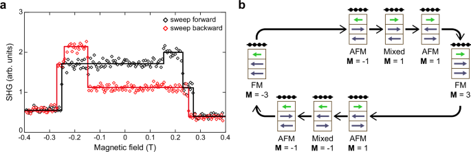
a SHG hysteresis loop measured using the excitation photon energy of 1.355 eV. b Magnetic evolution for the 3L CrSBr device. The electron doping from graphene (black dots and lines) modulates the contacted CrSBr layer, as indicated by green arrows.
Consequently, we outline the magnetic evolution of 3L CrSBr, as illustrated in Fig. 3b. In the forward sweep, the magnetic structure begins in the FM state (M = −3) under magnetic field of −0.4 T. As field sweeps to 0 T, a spin-flip transition occurs in the middle layer, driven by the interlayer AFM coupling from the two vdW interfaces, leading to the AFM state (M = −1). With further increases in magnetic field, the 3L CrSBr transitions to the Mixed state (M = 1). Notably, the charge transfer from graphene to 3L CrSBr leads to the reduction of the interlayer AFM coupling between the upper two CrSBr layers25, thereby promoting the formation of the Mixed state, in which the upper two layers become ferromagnetically coupled. In contrast, the spatial-inversion or time-reversal counterparts of this Mixed state, which require either flipping the bottom layer or simultaneously flipping the bottom two layers of the AFM state (M = −1) (Supplementary Table 1), remains energetically unfavorable under the sample geometry.
Subsequently, the trilayer CrSBr switches to the AFM state with M = 1 within a small field range near 0.25 T. This state is the time-reversal counterpart of the AFM state at 0 T (forward), which is intensity degenerate in PL measurements. The wavelength-dependent SHG measurements further distinguish these two states (Supplementary Fig. 5). Opposite transition behaviors are observed during the backward sweep from 0.4 T to −0.4 T, which exhibit a time-reversal evolution of the magnetic structures compared to the forward sweep. For comparison, an SHG loop of a bare 3L CrSBr is shown in Supplementary Fig. 6, which exhibits vanished SHG intensity due to the centrosymmetric magnetic structure of intrinsic AFM and FM states.
Gate-tunable magnetic transitions
The well-defined magnetic structures in the 3L CrSBr device allow us to study the magnetic transition behavior under variable gate voltages. Figure 4a displays the PL intensity loops across various gate voltages between ±60 V, with the magnetic field sweeps shown for both forward (upper panel) and backward (lower panel) directions. Interestingly, the transitions from the Mixed states to the FM states is significantly influenced by the gate voltages. Figure 4b, c present the zoomed-in magneto-PL data, focusing on the magnetic field range where the Mixed states switch to the FM states. Under positive gate voltages, the Mixed states transition directly to the FM states. By contrast, under negative gate voltages, the Mixed states undergo two-step transitions: first to the AFM states and then to the FM states. It is worth noting that the Fermi level of the graphene/3L CrSBr heterostructure is characterized to be nearly aligned with the Dirac point of the graphene (Supplementary Fig. 7). Accordingly, the CrSBr layer in contact with graphene is under the electron doping density of ~2.0 × 1013 cm−225,30, which arises from the Dirac point of graphene being ~0.5 eV higher than the conduction band minimum of CrSBr. In contrast, the maximum charge density induced by a 60 V back-gate voltage is only ~4.7×1012 cm−2, so that the CrSBr is always under the electron-doped regime throughout this study.
Fig. 4: Gate-tunable magnetic transitions for the 3L CrSBr device.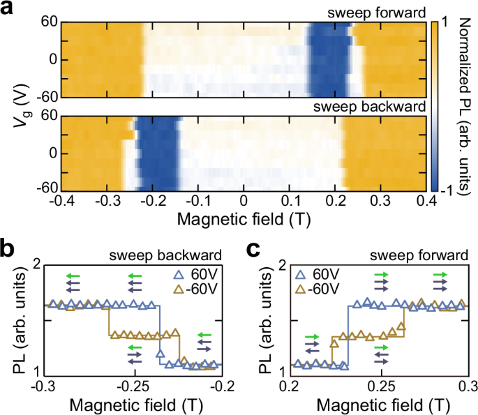
a Magneto-PL loops under different gate voltages. Zoomed-in PL intensity from the Mixed states to FM states during the backward (b) and forward (c) sweeps at Vg = ±60 V. The insets show the magnetic structures corresponding to the PL intensity plateaus. Compared to Vg = −60 V, the middle plateau corresponding to the AFM states disappears at Vg = 60 V.
To analyze the gate-controlled magnetic transitions, a simplified linear chain model is used to simulate the delicate energy balance within the magnetic evolution. In brief, the gate-controlled charge transfer effectively modulates the relative strength of interlayer exchange interactions, thereby tuning the spin-flipping sequence and determining the observed magnetic transition behavior (see details in Supplementary Note 3). For clarity, the three layers from the bottom to the top are labeled as layer 1, layer 2, and layer 3, respectively. The electrostatic doping in layer 3, which is induced by the gate voltage, modulates the interlayer exchange interaction \({J}_{23}\) between the top two CrSBr layers. Specifically, \({J}_{23}\) decreases under positive gate voltages and increases under negative voltages. At positive gate voltages, the reduction in \({J}_{23}\) allows the magnetic anisotropy energy \(K\) of layer 2 to play a dominant role in stabilizing its spin orientation. As a result, the 3L CrSBr device undergoes a direct transition from the Mixed state to the FM state, with only layer 1 flipping. By contrast, at negative gate voltages, the increased interlayer AFM coupling between layers 2 and 3 favors the simultaneous flipping of layers 1 and 2 before reaching the FM state. Consequently, an intermediate AFM state between the Mixed state and the FM state appears during the magnetic evolution.