Patent database
A comprehensive database was developed to analyze the spatial and temporal distribution of patent activity within a subset of contemporary U.S. patents spanning from 1905 to 2024. We identified eight high-impact innovation sectors, i.e., plug-in cars, fracking, end-user multimedia applications, video games, chip architectures, machine learning, biotechnology enzymes, and mobile devices-that play pivotal roles in driving technological progress and economic growth within the United States. The United States Patent and Trademark Office (USPTO) maintains a high-quality data source called PatentView39, which we have used to compile the database. Older patents (prior to 1976) were retrieved by manually downloading records from the USPTO’s public database (June 2024). This effort produced a unified, georeferenced patent dataset capturing contemporary technological trends across key innovative U.S. sectors, providing a valuable basis for both quantitative and spatial analyses of patent productivity over the past six decades. The resultant patent database comprises 139.387 USPTO patents.
For each patent, we collected detailed information, including the title, brief description, country of origin, assignee, names of inventors40, and geographic coordinates (latitude and longitude) of the first inventor’s location. To categorize patents by technology type, we first identified Cooperative Patent Classification (CPC) codes that correspond to each sector. CPC codes serve as a standardized method of classifying inventions based on their technical characteristics and applications. We assigned patents to technology sectors by searching the entire patent database for these CPC codes, which represent high-value innovation sectors. Each patent was categorized into a sector if it contained at least one relevant CPC code in its documentation. In the following, we describe each technological sector, its CPC code criteria, and its relevance in the U.S. innovation landscape.
The End-User Applications (24.165 patents with CPC code H04N 21/47) sector comprises patents for end-user multimedia applications characterized by their interactivity, service structure, and diverse functionalities. Relevant patents cover a wide range of services, from local multimedia applications to high-bandwidth uplink technologies, showcasing the growing influence of digital media in consumer technology.
The Plug-In Electric Cars (9.320 patents with CPC code: Y02T 90/14) sector encompasses patents related to plug-in electric vehicle technologies, which contribute to the development of sustainable transportation. These patents reflect innovation within the electric vehicle industry.
The Fracking (4.609 patents with CPC code: E21B 43/16) sector covers patents for enhanced hydrocarbon recovery methods, specifically hydraulic fracturing, used to mobilize hydrocarbons in reservoirs. Innovations in fracking technologies have transformed U.S. energy production and reshaped the nation’s role in global energy markets.
The Machine Learning (21.462 patents with CPC code: G06N 20/00) sector includes patents related to machine learning technologies, which equip machines with adaptive capabilities based on experiential data. These patents range from algorithms to physical machine implementations and reflect the transformative impact of artificial intelligence on diverse industries.
The Video Games (20.490 patents with CPC code: A63F 13/00) sector comprises patents encompassing a wide range of video game technologies, including hardware accessories, software innovations such as virtual camera animation, network-based game features, and cutting-edge game content generation, shaping the landscape of the video game industry and driving technological advancements. The dataset captures the technological complexity of modern electronic entertainment.
The Biotech Enzymes (51.853 patents with CPC code: C12Q) sector includes patents for processes involving enzymes, nucleic acids, and microorganisms, with applications in diagnostics and bioengineering. These patents reflect advances in healthcare, genomics, and environmental biotechnology, representing areas of life sciences innovation.
The Mobile Devices (2.108 patents with CPC code: H04M 1/0202) sector captures patents for portable telephones, including mobile phones and cordless handsets, specifically focusing on structural features of mobile devices. The growth of this sector illustrates the evolution of mobile communication and connectivity technologies.
The Chip Architecture (5.380 patents with CPC code: G06T 1/20) sector includes patents for graphics processors, including GPUs, pipelines, and architectures for image data processing. Patents in this sector are central to advancements in computer graphics, parallel processing, and the increasing performance demands of visual data applications.
Database reconstruction pipeline
The study recovers the patent database using a customized pipeline that combines many data sources and methods to deliver a complete georeferenced patent dataset. This reconstruction was designed to enable robust data collection, systematic processing, and integration of patent metadata (see Fig. 7a). First, by consolidating data from multiple sources, it ensures comprehensive coverage and minimizes biases inherent in individual datasets. Second, separating records based on temporal and classification differences allows for better handling of data heterogeneity, such as the pre-1976 and post-1976 patent formats. Lastly, the inclusion of georeferenced inventor locations supports the spatial multiscale analyses that are central to this study.
Fig. 7: Construction of the patent database.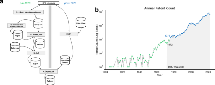
a This diagram summarizes the multi-stage reconstruction process used to build a spatially and sectorally resolved dataset of U.S. patents. The pipeline processes more than 4 million patents and extracts approximately 140,000 records across 8 technological domains. Two distinct workflows are implemented: one for pre-1976 patents (left side), which rely on scanned image records and OCR-based extraction, and another for post-1976 patents (right side), based on structured digital records. Both workflows include sector-specific keyword filtering, geolocation of assignees and inventors, and deduplication procedures (see “Methods”). b Annual counts of granted patents in the United States (1905–2024) are plotted on a logarithmic scale to emphasize long-term growth dynamics and visualize year-to-year variation across multiple orders of magnitude. The red dashed line indicates the year 1972, marking the threshold after which 99% of the total cumulative patents in the dataset were issued. The plot highlights the sharp rise in patenting activity over recent decades, which accounts for the majority of the dataset and motivates the focus on post-1970 dynamics in several analyses.
The process begins with data collection from three main platforms: (1) Patent View, (2) Dataverse, and (3) patents.google.com. Each of these sources contributes distinct datasets that complement one another. For instance, Google Patents provides raw patent records divided into pre-1976 and post-1976 periods to account for differences in archival formats. Patent View adds enriched metadata fields, while Dataverse contributes supplementary datasets such as classifications and regional identifiers. Semi-automated Python scripts were used to interact with these platforms, querying and downloading records based on patent identifiers.
Once the data is retrieved, parsing routines extract relevant information from the HTML files obtained from patents.google.com. This structured data includes fields such as patent titles, inventor locations, and classification codes, which are consolidated into an intermediate database labeled db1.
In the next stage, the database is refined by integrating additional fields from PatentView and Dataverse, such as CPC subgroup classifications (see above), geospatial coordinates, and temporal data. This step enhances data granularity and completeness, resulting in an updated database, db2, that contains both the parsed information and the enriched metadata.
Finally, the fully processed dataset is exported into a standardized CSV file, labeled full.csv, for use in subsequent analyses. This final export contains all fields necessary for the study, ensuring compatibility with statistical and geospatial analysis tools. The CSV format facilitates its use in a wide range of applications, from hierarchical clustering and spatio-temporal pattern analysis to inequality measurements.
Our analysis spans the time interval from 1905 to 2024; however, the bulk of the patent publications are concentrated in the last 52 years. As shown in Fig. 7b, the cumulative number of patents surpasses 99% of the total dataset starting from the year 1972.
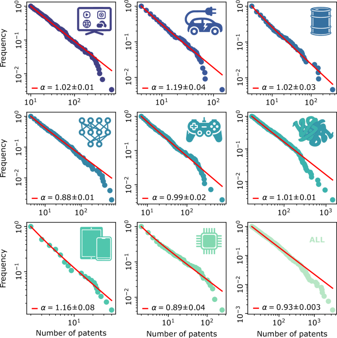
Fitting Zipf’s law
To investigate the heterogeneous distribution of patent activity across U.S. innovation sectors, we use Zipf’s law, a principle commonly used to analyze ranked distributions. Zipf’s law describes a situation where the frequency f(r) of an item is proportional to its rank r, expressed as
$$f(r) \sim {r}^{-\gamma },$$
(2)
where γ is the exponent characterizing the distribution. By plotting patent counts against rank on a log-log scale, we can assess whether patenting activity follows Zipf’s law across different geographic locations. For each sector, we ranked locations by patent count and fitted a power-law model using maximum likelihood estimation from the Python Powerlaw package version 1.541 (based on the work of Clauset et al.42), to evaluate if the observed rank-frequency distribution adheres to Zipf’s law or whether it can be best described by other distributions.
Analysis of size-conditional productivity
Temporal analysis of patenting activity reveals a two-phase pattern in the geographic diffusion of innovation. The initial phase is characterized by rapid spatial expansion, with each new patent frequently introducing a previously untapped location into the innovation network. This “boom” phase spans the emergence of the first 40–80 patents, regardless of technological domain (Fig. 2b), and is typically concentrated in established innovation hubs such as Silicon Valley (machine learning, software43,44), Houston (fracking45), and Boston (biotechnology46).
As patenting activity increases, the number of new entrants gradually decreases. Secondary hubs, such as Austin (electric vehicles47, gaming48) and Raleigh (biotechnology49,50), gradually enter the network, but do not displace the dominance of primary centers. The consistent temporal pattern shows that general principles, in combination with sector-specific dynamics51,52, shape the geography of innovation over time.
To quantify temporal dynamics, we analyze the size-conditional productivity of locations and the rate at which new locations enter the innovation network. We divide the patenting history into discrete time intervals, each containing 1/10th of the total patenting sequence, and measure patenting rates across these periods. Using a sliding window approach, we define a “present” bin containing 300 patents while considering all preceding patenting activity as the “past.”
For each location of size i (i.e., locations that had already produced i patents before the bin), we compute the normalized patenting productivity as:
$${P}_{i}=\frac{\Delta {N}_{i}}{\Delta N}$$
where ΔNi represents the increase in patent counts for locations of size i, and ΔN is the total number of patents in the interval. By removing P0 data (productivity associated with locations that had never produced a patent before), we characterize the cumulative advantage effect (Fig. 2a). Fitting a power-law relation to the empirical productivity values yields an estimated exponent γ = 0.962 ± 0.021, supporting the hypothesis that preferential attachment governs the growth of established innovation hubs.
In contrast, the entrant rate is quantified by measuring the fraction of patents associated with first-time entrants. Using sliding bins of 300 patents (with 25-patent step sizes), we track entrant rates over time across all eight technological sectors, obtaining an average trajectory.
To better understand the mechanisms driving these empirical trends, we consider two limiting cases in a stochastic innovation model: (1) the Scenario I (Constant Innovation Rate) assumes a fixed rate of new locations entering the innovation landscape. Under this scenario, diversity would grow linearly with the total number of patents, implying that patenting activity remains widely distributed without strong hub entrenchment; (2) the Scenario II (Resource-Limited Expansion) assumes that the system is bounded by an initial diversity pool, meaning that as patenting activity grows, new entrant opportunities diminish exponentially due to resource constraints and hub dominance.
To formalize these dynamics, we implement a stochastic model that simulates the evolution of the innovation landscape. The system begins with a pool of locations that have yet to produce patents. At each iteration, a location is selected based on cumulative advantage dynamics, meaning that locations with a strong history of innovation are more likely to continue patenting. When a patent is assigned, the location either already exists in the innovation network (reinforcing its status as a hub) or is a completely new entrant. Depending on the scenario, new locations are either introduced at a fixed rate (Scenario I) or drawn from a finite, resource-limited pool (Scenario II). Neither of these idealized cases fully captures the empirical patterns, as seen in Fig. 2b. The observed entrant rate declines sublinearly, following a power-law slowdown. This suggests that while innovation hubs consolidate their dominance over time, geographic expansion continues at a diminishing rate rather than abruptly ceasing53.
To examine how entrant dynamics influence the overall diversity of the innovation landscape, we track the temporal evolution of location diversity. If the system were purely resource-limited, diversity would saturate due to rapid entrant decay. Conversely, a constant-rate model would predict a steady increase in diversity. By tracking entrant rates and diversity growth under these conditions, we observe two contrasting behaviors. First, if new locations continue to emerge at a constant rate, diversity grows linearly with total patent output, and innovation remains widely distributed rather than being concentrated in hubs. And second, if location entry is resource-limited, diversity plateaus over time, and patenting activity becomes highly concentrated in a small number of dominant hubs.
Neither of these idealized cases fully captures empirical patterns, which instead exhibit a power-law slowdown in entrant rates and a long-term, sublinear increase in diversity (Fig. 2c). This suggests that while hub entrenchment is non-negligible, geographic expansion persists over long time scales, albeit at a diminishing rate.
Multiscale graph analysis
We develop a multiscale spatial framework that integrates geometric graph theory, percolation analysis, and fractal scaling to characterize the spatial organization of patenting activity. This approach quantifies how connected components of innovation emerge and how their structural properties vary with spatial resolution. Given a set of geolocated patents \({\mathcal{P}}={\{({x}_{i},{y}_{i})\}}_{i = 1}^{N}\), we deduplicate it to obtain L unique coordinates \({\mathcal{L}}={\{({x}_{j},{y}_{j})\}}_{i = 1}^{L}\), each with an associated weight Ni denoting the number of patents at that location. For each spatial scale R, we construct a geometric graph GR = (V, ER) where nodes represent unique locations and undirected edges connect nodes within distance R:
$${E}_{R}=\{(i,j)\in V\times V| \parallel ({x}_{i}-{x}_{j}){\parallel }_{2}\le R\}.$$
We compute the set of connected components \({Q}_{1},{Q}_{2},\ldots ,{Q}_{{n}_{R}}\) of GR, where each Qi contains all nodes linked through paths of edges not exceeding distance R. We define the “fragmentation function” as the fraction of connected components:
$$f(R)=\frac{{N}_{clusters}}{L}$$
(3)
where Nclusters is the number of connected components and L = ∣V∣ is the total number of nodes. This function tracks how the geometric graph fragmentation decreases as spatial proximity increases.
Empirical data exhibit a power-law decay in the fragmentation function:
$$f(R) \sim {R}^{-\beta },$$
(4)
indicating a scale-invariant, fractal-like structure in the spatial distribution of patenting36. This behavior contrasts with conventional spatial null models, where f(R) typically decays exponentially or exhibits a sharp percolation transition54,55. In the fractal regime–where the above scaling law holds–a single dominant connected component does not emerge, and patenting remains distributed across a hierarchy of spatial components. Although fractal patterns have been documented in urban geography30, the scaling observed in patenting networks emerges independently of population distribution, as demonstrated by the failure of population-based null models to reproduce the empirical (β) exponent (Fig. 3c–e).
To capture the full history of spatial aggregation, we track the merging of connected components across a range of radius thresholds and encode this information in a clustering tree. Initially, each node forms a singleton component. To efficiently identify spatial neighbors at each scale, we insert the points in \({\mathcal{L}}\) into a quadtree spatial index56. As R increases, overlapping connected components are merged, and these events are recorded as branches in a hierarchical tree. Each node in the clustering tree corresponds to a connected component, and merging events generate parent nodes from their child components. This structure preserves the complete multiscale aggregation history, enabling structural analyses of spatial organization. Figure 4a illustrates an example clustering tree whose hierarchical architecture is consistent across spatial scales. To assess the topological self-similarity of clustering trees, we adopt the shape tree analysis proposed by Herrada et al.32. For each region i, we define a subtree Si as the union of the connected component rooted at i and all its descendant regions. The size Ai is the total number of patents within Si, and the cumulative branch size Ci is:
$${C}_{i}=\sum _{j\in {S}_{i}}{A}_{j}.$$
(5)
This measure reflects the extent and asymmetry of spatial aggregation. Balanced trees minimize Ci, whereas more asymmetric or chain-like trees yield larger Ci values. Herrada et al. demonstrated that for many empirical trees, Ci and Ai satisfy an allometric scaling law:
$$C \sim {A}^{\tau },$$
(6)
with a universal exponent τ ≈ 1.44. We observe a similar exponent in the spatial organization of patenting (Fig. 4b), suggesting that the clustering trees obey similar scaling constraints to those found in biological or information networks. To further assess scale invariance, we examine the complementary cumulative distribution functions (CCDFs) of A and C:
$$F(A) \sim {A}^{1-{\tau }_{A}},\quad F(C) \sim {C}^{1-{\tau }_{C}},$$
(7)
both functions exhibit power-law tails (Fig. 4c), which supports the fractal nature of empirical clustering trees.
Coefficient of variation across scales
To explore whether spatial inequality in patenting exhibits scale dependence, we measure the coefficient of variation CV(R)-the ratio of standard deviation to mean of patent counts-across different aggregation scales R. Using the same geometric graph framework described above, we compute the connected components \({Q}_{1},{Q}_{2},\ldots ,{Q}_{{n}_{R}}\) at each spatial scale. The total patent count of component Qi is:
$${W}_{i}=\sum _{{v}_{j}\in {Q}_{i}}{N}_{j}.$$
From the set {Wi}, we compute:
$${\mu }_{R}=\frac{1}{{n}_{R}}\mathop{\sum }\limits_{i=1}^{{n}_{R}}{W}_{i},$$
$${\sigma }_{R}=\sqrt{\frac{1}{{n}_{R}}\mathop{\sum }\limits_{i=1}^{{n}_{R}}{({W}_{i}-{\mu }_{R})}^{2}},$$
and the coefficient of variation:
$$\,\text{CV}\,(R)=\frac{{\sigma }_{R}}{{\mu }_{R}}.$$
(8)
To assess robustness, we perform bootstrapping with 100 resampled datasets. The resulting confidence intervals (yellow curves in Fig. 5, top row) confirm that the observed peak in inequality is not an artifact of sampling variability, but rather a persistent feature of the spatial distribution of innovation. Our Python implementation automatically calculates the multiscale coefficient of variation CV(R) from a set of geographical locations.
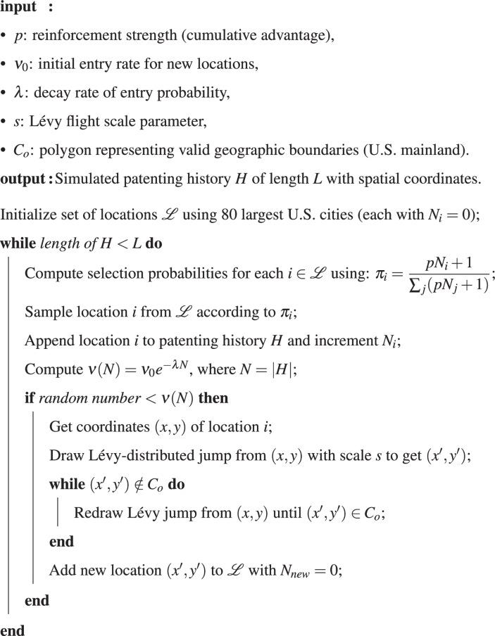
A stochastic model of innovation dynamics
To investigate the emergence of spatial patterns in U.S. patenting, we develop a minimal stochastic model that reproduces key empirical regularities described in Results. The model simulates the evolution of innovation activity through two fundamental processes: cumulative advantage and non-local dispersal.
The simulation unfolds over a geographic domain corresponding to the continental United States. It is initialized with the locations of the 80 most populous U.S. cities (population > 500,000), which act as potential starting points for innovation. At each time step, a new patent is added to the system. With some probability, the patent is assigned to an existing location i drawn from the current set \({\mathcal{L}}\) of active locations. The selection probability is given by a reinforcement mechanism:
$${\pi }_{i}=\frac{p{N}_{i}+1}{{\sum }_{j}(p{N}_{j}+1)},$$
(9)
where Ni is the cumulative number of patents at location i, and p controls the strength of cumulative advantage. This rule ensures that locations with a history of patenting activity are more likely to continue growing, reinforcing existing hubs over time12.
With probability ν(N), a new location is introduced instead. The rate of new location entry decays exponentially as the system matures:
$$\nu (N)={\nu }_{0}{e}^{-\lambda N},$$
(10)
where N is the total number of patents added so far, ν0 is the initial rate of entry, and λ controls the rate of decay. This reflects the empirically observed decline in new geographic entrants as existing hubs accumulate more patents (see Fig. 2c).
When a new location is added, its spatial coordinates are determined by a Lévy flight originating from the most recent location. Lévy flights combine frequent short steps with occasional long jumps and are widely used to model exploratory dynamics in spatially embedded systems57,58. Distances are sampled from a Lévy distribution (via scipy.stats.levy, with scale s = 0.1), and angles are drawn uniformly from [0, 2π). If the resulting location falls outside U.S. borders (defined by Co), the jump is repeated until a valid point is found using Natural Earth 110 m landmass shapefiles59.
The simulation proceeds for L iterations, producing a synthetic history of patenting locations and timestamps. This output is evaluated using the spatial methods introduced above?, including rank distributions, fractal clustering, and the coefficient of variation CV(R). By systematically varying parameters p and ν0, we map a continuous space of innovation regimes, from highly concentrated to widely dispersed systems (see Fig. 6b).
This model can be interpreted as a spatial urn process with reinforcement and exploration25. The pseudocode below summarizes the model’s implementation and variable definitions.
Algorithm 1
Stochastic model of patenting with reinforcement and Lévy dispersal
Analytical estimation of the inequality horizon
This section presents a macroscopic model for estimating the peak of spatial inequality in U.S. patenting activity-termed the inequality horizon (see above). The inequality horizon corresponds to the aggregation scale R* at which the coefficient of variation (CV) across patenting locations reaches its maximum.
The coefficient of variation, denoted CV(R), is defined as the ratio of the standard deviation σR to the mean μR of aggregated patent counts within clusters defined by a spatial radius R around each location. Modeling the behavior of μR and σR as a function of R is thus essential for understanding spatial inequality.
In the framework of Lévy geometric graphs (LGG)36, μR corresponds to the expected size of the connected component a node belongs to, given a connection radius R. For small R, most nodes remain isolated, and μR follows a power-law scaling:
$${\mu }_{R} \sim {R}^{a},$$
where a is a local aggregation exponent that quantifies the early-stage growth of clusters. Higher values of a indicate faster local connectivity, typically arising from dense short-range interactions. The value of a is influenced by the Lévy exponent s in the step-length distribution P(l) ~ l−s, where smaller s implies more spatial dispersion and suppressed local aggregation.
Unlike standard LGGs, the innovation dynamics modeled here include a reinforcement mechanism through node revisitation. At each time step, with probability 1 − ν, the process returns to an existing node (10), selected preferentially by accumulated patenting activity (9). This accelerates the growth of clusters relative to memoryless models, increasing the observed exponent a.
As R approaches a critical scale Rc, a percolation-like transition occurs, and μR diverges as:
$${\mu }_{R} \sim | {R}_{c}-R{| }^{-b},$$
where b is a divergence exponent characterizing the sharpness of the connectivity transition. Due to reinforcement, Rc tends to be lower than in standard LGGs, and the divergence can be steeper-potentially resembling explosive percolation60.
To describe the full range of R Rc, we propose the following unified scaling ansatz:
$${\mu }_{R}=c\,{R}^{a}| {R}_{c}-R{| }^{-b},$$
(11)
where c is a scale-dependent prefactor reflecting the overall density of innovation nodes. This expression captures both the early growth regime and the divergence near criticality. Figure 6g shows a least-squares fit of Eq. (11) to the simulation data.
Empirical analysis reveals that the standard deviation σR scales with the mean cluster size μR following a power-law relation:
$${\sigma }_{R} \sim {\mu }_{R}^{\delta },$$
(12)
where δ is the Taylor exponent, a measure of spatial heterogeneity. This form is equivalent to the classical Taylor’s law stated in terms of variance: Var ~ μ2δ. We adopt the standard deviation form for clarity and analytic convenience. In this formulation, δ = 1/2 corresponds to Poisson fluctuations; δ > 1/2 indicates clustering; and δ δ ≈ 3/4, suggesting nontrivial correlations.
While Eq. (12) holds asymptotically, empirical deviations occur at low μR due to sampling noise and finite-size effects. Figure 6g shows that σR initially grows slowly before transitioning to a power-law regime. To account for this behavior, we adopt a composite form:
$${\sigma }_{R} \sim {\mu }_{R}^{\delta }{\mathcal{M}}({\mu }_{R}),$$
(13)
where
$${\mathcal{M}}({\mu }_{R})=\frac{1}{1+\exp [-k({\mu }_{R}-{\mu }_{0})]}$$
(14)
is a logistic modulation term that suppresses variability for small cluster sizes (see inset in Fig. 6f). Here, μ0 sets the inflection point of the transition, and k controls its steepness.
This analytical framework applies for aggregation scales \(R > {R}_{\min }\approx 0.0{3}^{\circ }\) (approximately 3.3 km), above which spatial heterogeneity becomes scale-dependent. Below this threshold, empirical data show that CV(R) remains approximately constant (see Fig. 5), indicating a scale-invariant regime not captured by our model. This plateau suggests the presence of statistically homogeneous urban cores-consistent with longstanding urban design theories that define compact, walkable neighborhoods with diameters between 3 and 4 km33. These stable substructures likely reflect deeply rooted spatial organization in historical city planning and may serve as foundational units in the broader innovation landscape.
To obtain an analytic prediction for the inequality horizon, we approximate the logistic term with a rational function:
$${\mathcal{M}}({\mu }_{R}) \sim \frac{{\mu }_{R}}{{\mu }_{R}+{\mu }_{0}}.$$
Substituting this into Eq. (13) and dividing by μR gives an explicit expression for the coefficient of variation:
$${CV}(R)=\kappa \left(\frac{{\mu }_{R}^{\delta }}{{\mu }_{R}+{\mu }_{0}}\right),$$
(15)
where κ is a constant of proportionality.
To find the scale R* that maximizes CV(R), we treat μR = μ as the independent variable and set the derivative to zero:
$$\frac{d\,{CV}}{d\mu }=\kappa \frac{d}{d\mu }\left(\frac{{\mu }^{\delta }}{\mu +{\mu }_{0}}\right)=0.$$
Applying the quotient rule:
$$\frac{d\,{CV}}{d\mu }=\kappa \frac{\delta {\mu }^{\delta -1}(\mu +{\mu }_{0})-{\mu }^{\delta }}{{(\mu +{\mu }_{0})}^{2}}.$$
Setting the numerator to zero and dividing both sides by μδ−1:
$$\delta (\mu +{\mu }_{0})-\mu =0.$$
Solving for μ gives the critical mean cluster size:
$${\mu }^{* }={\mu }_{0}\left(\frac{\delta }{1-\delta }\right).$$
Substituting μR for clarity:
$${\mu }_{R}^{* }={\mu }_{0}\left(\frac{\delta }{1-\delta }\right).$$
(16)
This condition holds only if δ δ ≥ 1, spatial heterogeneity grows faster than mean aggregation, and CV(R) increases monotonically toward the percolation threshold.
Given the parametric form of μR in Eq. (11), we can numerically invert \({\mu }_{R}^{* }\) to find the corresponding inequality horizon R*. The parameters a, b, c, Rc, δ, μ0, and κ are fit to empirical data using nonlinear regression. Our Python code implements this procedure and provides theoretical estimates of the inequality horizon for any spatially distributed dataset of innovation activity.